1: 1次元変数変換
定理:変数変換と確率密度関数
定理
確率変数 \(X\) の確率密度関数を\(f_X(x)\)とし、 \(Y = g(X)\)とする. \(g(\cdot)\)が単調増加もしくは単調減少な関数とし、\(g^{-1}(y)\)が微分可能であるとき、
\[f_Y(y) = f_X(g^{-1}(y))\left|\frac{d}{dy}g^{-1}(y)\right| = f_X(g^{-1}(y))\left|\frac{1}{g'(g^{-1}(y))}\right| \tag{1.1}\]■
直感的説明
連続型確率変数 $X$, 関数 $g(\cdot)$, $Y = g(X)$としたとき、\(Y\) の確率密度関数を導きたいとします.分布関数\(F_Y(y)\)は
\[\begin{aligned} F_Y(y) &= P(g(X)\leq y)\\ &= P(X\in \{x\mid g(x)\leq y\}) \end{aligned}\]$Y$の確率密度関数は、$F_Y(y)$の$y$に対する一次導関数で導けるので、
\[\begin{aligned} f_Y(y) &= \frac{d}{dy}F_Y(y) \\ & = \frac{d}{dy}P(X\in \{x\mid g(x)\leq y\}) \end{aligned}\]特に、\(g(\cdot)\)が単調増加関数のときには、\(g(\cdot)\)の逆関数\(g^{-1}(\cdot)\)が存在することから、
\[\{x\mid g(x)\leq y\} = \{x\mid x\leq g^{-1}(y)\}\]従って、
\[F_Y(y) = \int^{g^{-1}(y)}_{-\infty}f_X(x)dx\]確率密度関数は
\[f_Y(y) = f_X(g^{-1}(y))\frac{d}{dy}g^{-1}(y)\]ここで、\(g(g^{-1}(y)) = y\)の両辺を\(y\)で微分すると
\[g'(g^{-1}(y))\frac{d}{dy}g^{-1}(y) = 1\]なので
\[f_Y(y) = f_X(g^{-1}(y))\frac{1}{g'(g^{-1}(y))}\]■
命題:累積分布関数と一様分布
命題
連続型確率変数 \(X\) の分布関数を\(F_X(x)\) とし、新たに確率変数 \(Y\) を \(Y = F_X(X)\) で定義する.このとき
\[Y \sim \mathrm{U}(0, 1)\]証明
区間\(y \in (0, 1)\)に対して、\(F_X(x)\)は単調増加関数. 従って、
\[\begin{aligned} F_Y(y) &= P(F_X(X)\leq y)\\ &= P(X\leq F^{-1}_X(y))\\ &= F_X(F^{-1}_X(y)) \end{aligned}\]両辺を\(y\)で微分すると
\[f_Y(y) = f_X(F^{-1}_X(y))\frac{1}{f_X(F^{-1}_X(y))} = 1\]従って、\(Y \sim \mathrm{U}(0, 1)\)となることがわかる.
■
定理:確率変数の線形変換
連続型確率変数 \(Z\) の確率密度関数が \(f_Z(z)\)で与えられているとします. \(\mu\)を実数, \(\sigma\)を正の実数とし
\[X = \sigma Z + \mu \tag{1.2}\]としたとき、\(X\)の確率密度関数は
\[f_X(x) = \frac{1}{\sigma}f_Z\left(\frac{x-\mu}{\sigma}\right)\]証明
(1.1)に(1.2)を代入すると
\[f_X(x) = f_Z\left(\frac{X - \mu}{\sigma}\right)\frac{1}{\sigma}\]■
練習問題
(1) 平方変換
連続型確率変数 $Z$ の確率密度関数が $f(z)$で与えられているとする.
\[X = Z^2\]としたとき、$X$の確率密度関数は
\[\begin{aligned} F_X(x) &= P(Z^2 \leq x)\\ &= P(-\sqrt{x} \leq Z \leq \sqrt{x})\\ &= F_Z(\sqrt{x}) - F_Z(-\sqrt{x}) \end{aligned}\]従って、
\[\begin{align*} f_X(x) &= \frac{d}{dx}F_Z(\sqrt{x}) - F_Z(-\sqrt{x})\\ &= \frac{1}{2\sqrt{x}}f_Z(\sqrt{x}) + \frac{1}{2\sqrt{x}}f_Z(-\sqrt{x}) \\ &= (f_Z(\sqrt{x}) + f_Z(-\sqrt{x}))\frac{1}{2\sqrt{x}} \tag{1.3} \end{align*}\]■
(2) 平方変換から平均と分散を求める
確率変数 \(X\) の確率密度関数が
\[f(x) = \frac{1 + x}{2}, \: \text{s.t. } x \in (-1, 1)\]で与えられているとき、変数変換 \(Y = X^2\) の確率密度関数と平均と分散を求めたいとします.
\[\int^{1}_{-1} \frac{1 + x}{2} dx = \left[\frac{1}{4}(1 + x)^2\right]^1_{-1} = 1\]解答
より確率密度関数の条件を満たしていることがわかります. 次に(1.3)と照らし合わせると,確率密度関数は
\[f_Y(y) = \frac{1}{2}\frac{1}{\sqrt{y}}(f_X(\sqrt{y})+f_X(-\sqrt{y})) = \frac{1}{2\sqrt{y}}\]次に、平均と分散を求めます
\[\begin{align*} E[Y] &= \int^1_0\frac{1}{2}y\frac{1}{\sqrt{y}}dy\\ &= \frac{1}{2}\int^1_0\sqrt{y}dy\\ &= \frac{1}{3}\\ E[Y^2] &= \int^1_0\frac{1}{2}y^2\frac{1}{\sqrt{y}}dy\\ &= \frac{1}{2}\int^1_0 y^{\frac{3}{2}}dy\\ &= \frac{1}{5} \end{align*}\] \[\therefore \: Var(Y) = \frac{1}{5} - \frac{1}{9} = \frac{4}{45}\]Pythonで確認してみる
方針
- $(0, 1)$区間の一様乱数を発生させる
- 逆関数法を用いて、$F_X(x)$に従う乱数を生成する
Libraries
1
2
3
import random
import numpy as np
import matplotlib.pyplot as plt
Classと関数の定義
1
2
3
4
5
6
7
8
9
10
11
12
13
14
15
16
17
18
19
20
21
22
23
24
25
26
27
28
29
30
31
32
33
34
35
36
37
38
39
40
41
42
43
44
45
46
47
48
49
50
51
52
53
54
55
56
57
58
59
60
61
62
class SampleGenerator:
    def __init__(self, sample_size, seed = 42):
        self.sample_size = sample_size
        self.seed = seed

    def random_sampling(self):
        """
        Return random samples which follows the density function:
          f(x) = (1 + x)/2 where x in (-1, 1) else 0

        And

        Return Y = X^2
        """
        random.seed(self.seed)
        self.data = [self.inv_cumulative(random.uniform(0, 1)) for i in range(self.sample_size)]
        self.transformed_data = [i**2 for i in self.data]

    def describe(self, transformed = None):
        """
        Reutrn the mean and variable of the data

        Note
          the variance is based on the unbiased variance
        """
        if transformed:
            tmp_data = self.transformed_data
        else:
            tmp_data = self.data

        mean, var =  np.mean(self.data), np.var(tmp_data, ddof = 1)
        print("the mean: {}\nthe variance: {}".format(mean, var))

    @staticmethod
    def inv_cumulative(prob):
        """
        the density function:
          f(x) = (1 + x)/2 where x in (-1, 1) else 0

        the cumulative function
          F(x) = (1 + x)^2/4 where x in (-1, 1)
            if x <= -1 then 0
            if x >= 1 then 1
        """

        return 2 * prob ** 0.5 - 1

def x_density(x):
    """
    the density function:
        f(x) = (1 + x)/2 where x in (-1, 1) else 0
    """

    return (1 + x)/2

def y_density(y):
    """
    the density function:
        f(y) = 1/(2 * y**0.5) else 0
    """

    return 1/(2 * y**0.5)
平均と分散の確認
1
2
3
4
5
6
7
8
Experiment = SampleGenerator(10000)
Experiment.random_sampling()

print("the original data")
Experiment.describe()

print("\nthe transformed data")
Experiment.describe(transformed=1)
Then,
1
2
3
4
5
6
7
the original data
the mean: 0.3346733874809254
the variance: 0.21967269701823616

the transformed data
the mean: 0.3346733874809254
the variance: 0.08801896143609267
上の計算結果とほぼ一致する結果が確認できました.
XとYの分布の確認
まず確率変数 \(X\) の分布を確認します
1
2
3
4
5
6
7
8
9
10
fig, ax = plt.subplots(1, 1,figsize=(10, 10))

xgrid = np.linspace(-1, 1, 200)

ax.hist(Experiment.data, density = True, bins = 100, label = 'sampling')
ax.plot(xgrid, x_density(xgrid),lw=2, color='#A60628',label = 'True density')
ax.set_title('density function: $f(x) = (1 + x)/2$', fontsize=15)
ax.set_xlabel('x value', fontsize=12)
ax.set_ylabel('density', fontsize=12)
ax.legend(fontsize=12);

つぎに同様のコードを実行して \(Y\)の分布を確認します

(3) 平方変換と絶対値を用いた確率密度関数
$X$を連続型確率変数で、その確率密度関数が
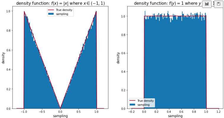
\[f_X(x) = \begin{cases} |x| & x \in [-1, 1)\\ 0 & otherwise \end{cases}\]このとき, $Y = X^2$の確率密度関数は(1.3)より $f_Y(y )= 1 \text{ where } y \in [0, 1]$
Python
1
2
3
4
5
6
7
8
9
10
11
12
13
14
15
16
17
18
19
20
21
22
23
24
25
26
27
28
29
30
31
32
33
34
35
36
37
38
39
40
41
42
43
44
45
46
47
48
49
50
51
52
53
54
55
56
57
58
59
60
61
62
63
64
65
66
67
68
69
70
71
72
73
74
75
76
77
78
79
80
81
82
83
## Library
import random
import numpy as np
import matplotlib.pyplot as plt
from statsmodels.distributions.empirical_distribution import ECDF

## Class and methods
class SampleGenerator:
    def __init__(self, sample_size, seed = 42):
        self.sample_size = sample_size
        self.seed = seed

    def random_sampling(self):
        """
        Return random samples which follows the density function:
          f(x) = |x| where x in (-1, 1) else 0

        And

        Return Y = X^2
        """
        random.seed(self.seed)
        self.data = [self.inv_cumulative(random.uniform(0, 1)) for i in range(self.sample_size)]
        self.transformed_data = [i**2 for i in self.data]

    def describe(self, transformed = None):
        """
        Reutrn the mean and variable of the data

        Note
          the variance is based on the unbiased variance
        """
        if transformed:
            tmp_data = self.transformed_data
        else:
            tmp_data = self.data

        mean, var =  np.mean(tmp_data), np.var(tmp_data, ddof = 1)
        print("the mean: %.3f\nthe variance: %.3f" % (mean, var))

    @staticmethod
    def inv_cumulative(prob):
        """
        the density function:
          f(x) = |x| in (-1, 1) else 0
        """
        x = None
        if prob > 0.5:
            x = (2 * (prob - 0.5)) ** 0.5
        else:
            x = -(-2 * (prob - 0.5)) ** 0.5

        return x

def x_density(x):
    """
    the density function:
        f(x) = |x| where x in (-1, 1) else 0
    """

    return abs(x) if -1 <= x <= 1 else 0

def y_density(y):
    """
    the density function:
        f(y) = 1 wehre y in (0, 1) else 0
    """
    dens_y = 1 if 0 <= y <= 1 else 0

    return dens_y

def plot_simulation(data, grid, density_func, title, xlabel, ax = None):
    dens_vec = np.vectorize(density_func, otypes=[np.float64])

    if ax is None:
        fig, ax = plt.subplots(1, 1,figsize=(10, 7))

    ax.hist(data, density = True, bins = 100, label = 'sampling')
    ax.plot(grid, dens_vec(grid),lw=2, color='#A60628',label = 'True density')
    ax.set_title(title, fontsize=15)
    ax.set_xlabel(xlabel, fontsize=12)
    ax.set_ylabel('density', fontsize=12)
    ax.legend()
変数変換前と変数変換後のmean, varを出力してみると
1
2
3
4
5
6
7
8
9
10
11
12
13
14
15
16
Experiment = SampleGenerator(100000)
Experiment.random_sampling()

print("the original data")
Experiment.describe()

print("\nthe transformed data")
Experiment.describe(transformed=1)

>> the original data
>> the mean: 0.001
>> the variance: 0.501
>>
>> the transformed data
>> the mean: 0.501
>> the variance: 0.083
またランダムサンプリング及び変数変換後の分布をplotで確認してみます.
1
2
3
4
5
6
7
8
9
10
11
12
13
14
15
16
17
18
19
xgrid = np.linspace(-1.2, 1.2, 200)
ygrid = np.linspace(-0.2, 1.2, 200)
fig, ax = plt.subplots(1, 2,figsize=(14, 7))

plot_simulation(data = Experiment.data,
                grid = xgrid,
                density_func = x_density,
                xlabel= 'sampling',
                title = 'density function: $f(x) = |x|$ where $x \in (-1, 1)$',
                ax = ax[0])


plot_simulation(data = Experiment.transformed_data,
                grid = ygrid,
                density_func = y_density,
                xlabel= 'sampling',
                title = 'density function: $f(y) = 1$ where $y \in (0, 1)$',
                ax = ax[1])
(4) Truncated Distribution
問題
確率密度関数 $f(x)$ と分布関数 $F(x)$ について、適当に実数 $a$ をとって関数 $g(x)$ を
\[g(x) = \begin{cases} f(x)/(1 - F(a)) & x > a\\ 0 & \text{ otherwise } \end{cases}\]この関数をtruncated distributionといいます. これが確率密度関数になることを示します.
解答
定義から
\[g(x) = f(x)/(1 - F(a))I(x>a)\]なので、$g(x) \geq 0$ と $\int_a^\infty f(x)/(1 - F(a))I(x>a) dx = 1$は自明. 従って、$g(x)$は確率密度関数になっている.
\[f(x) = \begin{cases} \exp(-x) & x > 0\\ 0 & \text{ otherwise } \end{cases}\]例
としたとき、$a = 1$のときの$g(x)$を考えたいと思います.
上記の確率密度関数が与えられた時の$F(a)$は
\[\begin{aligned} F(a) &= \int^a_0 \exp(-x) dx\\ &= [-\exp(-x)]^a_0\\ &= 1 - \exp(-a) \end{aligned}\]なので
\[\begin{aligned} g(x) &= \frac{\exp(-x)}{\exp(-a)}\\ & \exp(a - x) \end{aligned}\]これに $a=1$を代入すると、$g(x) = \exp(1-x)$
\[\begin{aligned} F(x) &= 1 - \exp(-x)\\ F^{-1}(F(x)) &= -\log(1 - F(x)) = x \end{aligned}\]Python Simulation
これに注意すると、「(2) 平方変換と絶対値を用いた確率密度関数」で用いたクラスを以下のように修正.
1
2
3
4
5
6
7
8
9
10
11
12
13
14
15
16
17
    def random_sampling(self):
        random.seed(self.seed)
        self.data = [self.inv_cumulative(random.uniform(0, 1)) for i in range(self.sample_size)]
        self.transformed_data = list(filter(lambda x: x >= 1, self.data))

    @staticmethod
    def inv_cumulative(prob):
        x = - np.log(1 - prob)

        return x

def x_density(x):

    return np.exp(-x)

def y_density(y):
    return np.exp(1-y) if y >= 1 else 0

(5) 標準正規分布に従う確率変数の指数変換
$X \sim N(0, 1)$のとき, $Y= \exp(X)$の確率密度関数を求めよ
解答
$\exp(\cdot)$は連続な単調増加関数で逆関数 $X = \log (Y)$をもつ. 従って、
\[F_Y(y) = F_X(\log (y))\]両辺を$y$で微分すると
\[\begin{aligned} f_Y(y) &= f_X(\log(y))\frac{1}{y}\\ &= \frac{1}{\sqrt{2\pi}}\exp\left(-\frac{(\log y)^2}{2}\right)\frac{1}{y} \: (t\leq 0) \end{aligned}\]$E[y], E[y^2]$は
\[\begin{aligned} \int_0^\infty \frac{1}{\sqrt{2\pi}}\exp\left(-\frac{(\ln y)^2}{2}\right) dy & = \sqrt{e}\\ \int_0^\infty \frac{1}{\sqrt{2\pi}}\exp\left(-\frac{(\ln y)^2}{2}\right) dy & = e^2 \end{aligned}\]と計算されます. 実際にPythonで確認してみると
1
2
3
4
5
6
7
np.random.seed(42)
x = np.exp(np.random.normal(0, 1, 100000))
print(np.mean(x))
print(np.mean(x**2))

>>>1.6504022457562608
>>>7.323861940067089
と近い値が出力されることが確認できます.
(6) 区間によって単調変換ができない場合の変数変換
確率変数 $X$ の密度関数が
\[f_X(x) = \frac{2}{9}(x + 1) \: -1 \leq x \leq 2\]で与えられているとき、$Y = X^2$の密度関数を求めたいとします
解答
$0 < y < 1\(と\)1 \leq y < 4$ に分けて考える.
前者について、
\[f_Y(y) = \frac{1}{2\sqrt{y}}(f_X(\sqrt{y}) + f_X(-\sqrt{y})) = \frac{2}{9\sqrt{y}}\]後者については、1 対 1 変換となることに注意すると
\[\begin{aligned} F_Y(y) &= P(X^2 \leq 1) + P(1 < X^2 \leq y)\\ &= \frac{2}{9}\int^{1}_{-1}(1 + x)dx + P(1 < X^2 \leq y)\\ &= \frac{4}{9} + \int^{\sqrt{y}}_1\frac{2}{9}(1+x)dx\\ &= \frac{1}{9} + \frac{1}{9}(y + 2\sqrt{y}) \end{aligned}\]従って、$y$で両辺を微分すればよいので
\[f_Y(y) = \frac{1}{9}\left(1 + \frac{1}{\sqrt{y}}\right)\]まとめると、
\[f_Y(y) = \begin{cases} \frac{2}{9\sqrt{y}} & \: 0 < y < 1\\ \frac{1}{9}\left(1 + \frac{1}{\sqrt{y}}\right)& \: 1 \leq y < 4 \end{cases}\]■
Simulation with Python
今回の $X$の累積分布関数は
\[F_X(x) = \frac{1}{9}(x + 1)^2\]なので
\[F_X^{-1}(p) = 3\sqrt{p} - 1\]- Pythonでsimulationはこちら
2: 2次元変数変換
変数変換の公式
$(X, Y)$を確率変数とし、$S = g_1(X, Y), T = g_2(X, Y)$ なる変数変換を考えます. $\mathbf R^2$上の集合Dに対して、
\[C = \{(x, y)| (g_1(x, y), g_2(x, y))\in D\}\]とするとき
\[P((S, T)\in D) = P((X, Y)\in C)\tag{2.1}\]を考えることができます.
離散型確率変数の場合
$C_{u, v} = {(x, y)| g_1(x, y) = u, g_2(x, y)= v}$とおくと、$(S, T)$の同時確率関数は
\[f_{S, T}(u, v) = P((X, Y)\in C_{u,v}) = \sum_{(x, y)\in C_{u,v}}f_{X, Y}(x, y)\tag{2.2}\]連続型確率変数の場合
基本方針は(2.2)と同じ形となります. 特に$(X, Y)$と$(S, T)$の対応が1対1対応の場合,$(S, T)$の確率密度関数を陽に表現することができます. まず最初に$(X, Y)$と$(S, T)$の対応が以下のように表現されるとします.
\[\begin{aligned} X &= h_1(S, T)\\ Y &= h_2(S, T) \end{aligned}\]次にヤコビアンを定義します.
\(\begin{aligned} J(s, t) &= J((s, t)\to(x, y))\\ &= \text{det}\left(\begin{array}{cc} \frac{\partial h_1(s, t)}{\partial s} & \frac{\partial h_1(s, t)}{\partial t}\\ \frac{\partial h_2(s, t)}{\partial s} & \frac{\partial h_2(s, t)}{\partial t} \end{array}\right) \end{aligned}\)
このとき、重積分の変数変換公式より
\(\int\int_{(x, y)\in C}f_{X, Y}(x, y)dxdy = \int\int_{(S, T)\in D}f_{X, Y}(h_1(s, t), h_2(s, t))|J(s, t)|dsdt\)
また、ヤコビアン $J((s, t)\to(x, y))$は以下の関係も有する:
\[J((s, t)\to(x, y)) = \frac{1}{J((x, y)\to(s, t))}\]確率変数の和の分布
2つの確率変数 $X, Y$が独立に分布し$X\sim f_X(x)$, $Y\sim f_Y(y)$としたとき、 $Z =X+Y$の分布を求めたいとします. これは変数変換によって確認することができます.
まず、
\[\begin{align*} Z & = X+Y\\ T &= Y \end{align*}\]という変数変換を考えます. このときの$(Z, T)$の同時確率密度関数は
\[f_{Z,T}(z, t) =f_X(Z-t)f_y(t)\quad\quad\tag{2.3}\]Zの分布は(2.1)の周辺分布で与えられるので
\[f_Z(z) = \int f_X(Z-t)f_y(t)dt \quad\quad\tag{2.4}\]これを$f_X$と$f_Y$の畳み込み(convolution)といいます.
$X, Y$が共に正規分布に従うとき
\[\begin{align*} X&\sim N(\mu_X, \sigma_X^2)\\ Y&\sim N(\mu_Y, \sigma_Y^2) \end{align*}\]のとき、$Z = X + Y$の密度関数を導出したいとします. (2.4)より
\(f_Z(z) = \frac{1}{\sqrt{2\pi(\sigma_X^2+\sigma_Y^2)}}\exp\left(\frac{z - \mu_X - \mu_Y}{2(\sigma_X^2+\sigma_Y^2)}\right) \int \frac{1}{\sqrt{2\pi (\sigma_X^2\sigma_Y^2)/(\sigma_X^2+\sigma_Y^2)}}\exp\left(-\frac{(t - (\sigma^2_Y(z - \mu_X) - \sigma^2_X\mu_Y)/(\sigma_X^2+\sigma_Y^2))^2}{2(\sigma_X^2\sigma_Y^2)/(\sigma_X^2+\sigma_Y^2)}\right)\)
従って、積分の中身は正規分布の密度関数の形をしているので
\[f_Z(z) = \frac{1}{\sqrt{2\pi(\sigma_X^2+\sigma_Y^2)}}\exp\left(\frac{z - \mu_X - \mu_Y}{2(\sigma_X^2+\sigma_Y^2)}\right)\]従って、$Z\sim N(\mu_X+\mu_Y, \sigma_X^2+\sigma_Y^2)$
練習問題
(2-1) 指数分布と変数変換: 2019年11月統計検定1級より
問題
確率変数 $X_1, X_2$は互いに独立に指数分布に従うとします
\[f(x) = \lambda \exp(-\lambda x) \ \ \text{ s.t } x > 0,\lambda > 0\]それらの和を $S = X_1 + X_2$, 標本平均を $\bar X = S/2$とします. このとき、以下の設問を答えよ.
- $E[S]$をもとめよ
- $S$ の確率密度関数 $g(s)$ をもよめよ
- $E[1/S]$をもとめよ
- $\alpha$ を正の定数とし、パラメーター $\theta \equiv 1/\lambda$を $\alpha \bar X$で推定します. その時の損失関数を
として期待値 $R(\alpha, \theta) \equiv E[L(\alpha \bar X, \theta)]$を導出せよ. また、左の期待値が最小となる $\alpha$ の値も求めよ.
解答 (1)
確率変数 $X_1, X_2$は互いに独立に指数分布に従うので
\[E[S] = E[X_1 + X_2] = E[X_1] + E[X_2]\] \[\begin{aligned} E[X_1] &= \int_0^\infty x\lambda \exp(-\lambda x)dx\\ &= [-x\exp(-\lambda x)]^\infty_0 + \int_0^\infty \exp(-\lambda x)dx\\ &= \frac{1}{\lambda} \end{aligned}\]従って, $E[S] = 2/\lambda$
解答 (2): 畳み込み, convolution
$(X_1, X_2)\to(S, T)$への変数変換を以下のように考えます
\[\begin{aligned} S &= X_1 + X_2\\ T &= X_1 \end{aligned}\]逆変換は
\[\begin{aligned} X_1 &= T\\ X_2 &= S - T \end{aligned}\]これにより、(S, T)の同時確率密度関数は $t > 0, s - t > 0$ に注意して
\[g(s, t) = f(t)f(s - t)|J| = \lambda^2 \exp(-\lambda s)\]よって, $s - t$を $(0, s)$区間で積分すれば $g(s)$が得られるので
\[g(s) = \int_0^{s}\lambda^2 \exp(-\lambda s)dt = \lambda^2 s \exp(-\lambda s)\]\[\begin{aligned} E[1/S] &= \int_0^\infty \frac{1}{s}\lambda^2 s \exp(-\lambda s) ds\\ &= \lambda \end{aligned}\]解答 (3)
解答(4)
(1)と(3)より
\[\begin{aligned} R(\alpha, \theta) &= E\left[\frac{\alpha \bar X}{\theta} + \frac{\theta}{\alpha \bar X}-2\right]\\ &= \frac{\alpha}{\theta}E[\bar X] + \frac{\theta}{\alpha}E[1/\bar X] - 2\\ &= \alpha + \frac{1}{\alpha} - 2 \end{aligned}\]「$\alpha$ を正の定数」という条件より、$\alpha$の定義域において、これは連続関数なので$\alpha$で微分して0となる数値が局地となります. また、二階条件が正となれば、その局地は最小値をとるので
\[\begin{aligned} R'(\alpha) &= 1 - 2/\alpha^2\\ R''(\alpha) &= 4/\alpha^3 > 0 \end{aligned}\]従って、$\alpha = \sqrt {2}$で$R(\alpha)$は最小値を取る.
(2-2) 標準正規分布と極座標変換
$X, Y$が独立に標準正規分布に従うとします. このとき以下の変数変換を考えます.
\(\begin{align*} X & = r\cos\theta\\ Y & = r\sin\theta \end{align*}\)
$(r, \theta)$の同時確率密度関数及び、それぞれの確率密度関数をもとめよ.
解答: $(r, \theta)$の同時確率密度関数
$(r, \theta)\to (X, Y)$のヤコビアンは
\(J((r, \theta)\to (X, Y)) = \left|\text{det}\left(\begin{array}{cc} \cos\theta & -r\sin\theta\\ \sin\theta & r\cos\theta \end{array}\right)\right| = r\)
従って, $r\in (0, \infty), \theta\in(0, 2\pi)$に注意して
\(\begin{align*} f_{r, \theta}(r, \theta)&= f_{X, Y}(r\cos\theta, r\sin\theta)r\\ &= f_{X}(r\cos\theta)f_Y(r\sin\theta)r\\ &= \frac{1}{2\pi}r\exp(-r^2/2) \end{align*}\)
解答: $(r, \theta)$のそれぞれの確率密度関数
$\int_0^\infty r\exp(-r^2/2)dr = 1$であることに留意すると、$(r, \theta)$は独立に分布し、
\(\begin{align*} r&\sim r\exp(-r^2/2)\\ \theta&\sim U(0, s\pi) \end{align*}\)
Python: $r, \theta$の理論分布と変数変換結果のqq-plot比較
まず、$r, \theta$を陽に表すと
\(\begin{align*} r & = \sqrt(X^2 + Y^2)\\ \theta &= 2(\arctan((- \sqrt(X^2 + Y^2) - X)/Y) + \pi/2) \end{align*}\)
従って、
1
2
3
4
5
6
7
8
9
10
11
12
13
14
15
16
17
18
19
20
21
22
23
24
25
26
27
28
29
30
31
32
33
34
35
36
37
38
39
40
41
42
43
44
45
46
47
48
49
50
51
52
53
54
55
56
57
58
59
60
61
62
63
64
65
## Data generation
N = 10000
np.random.seed(42)
X, Y = np.random.normal(0, 1, N),np.random.normal(0, 1, N)

r = np.sqrt(X**2 + Y**2)
theta = 2*(np.arctan((- np.sqrt(X**2 + Y**2) - X)/Y) + np.pi/2)

## 理論分布に基づくsampling
def inverse_cdf_r(prob):
    return np.sqrt(-2 * np.log(1 - prob))

prob_range = np.random.uniform(0, 1, N)
r_true = inverse_cdf_r(prob_range)
theta_true = np.random.uniform(0, 2*np.pi, N)

## qqplot
def qqplot(x, y, title = None, xlabel = None, ylabel = None, plot = False, ax = None):
    """
    INPUT
        x, y : array_like, 1-Dimensional
            Two arrays of sample observations

    Returns:
        statistic: float
            KS statistic.
        pvalue: float
            One-tailed or two-tailed p-value.
        Figure:
            QQ-plot
            x-axis and y-axis is normalized between 0 and 1
    """

    sorted_x = sorted(x)
    x_xdf, y_cdf = ECDF(x), ECDF(y)
    ks_test = stats.ks_2samp(x, y)

    print(ks_test)

    if ax is None:
        fig, ax = plt.subplots(1, 1,figsize=(9, 9))

    if plot:
        ax.plot(x_xdf(sorted_x), y_cdf(sorted_x),lw=2, color='#0485d1')
    else:
        ax.scatter(x_xdf(sorted_x), y_cdf(sorted_x),lw=2, color='#0485d1')

    ax.axline([0, 0], [1, 1],lw=4, color='#A60628')
    ax.set_title(title  + '  (ks-test p-value: %.3f )'%ks_test[1] , fontsize=15)
    ax.set_xlabel(xlabel, fontsize=13)
    ax.set_ylabel(ylabel, fontsize=13)
    plt.legend()

## qqplot
qqplot(r, r_true,
        title = 'QQ-plot between r and true r',
        xlabel = r'$r$ from transformation',
        ylabel = 'sampling from pdf $r\exp(-r^2/2)$',
        ax = None)

qqplot(theta, theta_true,
        title = r'QQ-plot between $\theta$ and true $\theta$',
        xlabel = r'$\theta$ from transformation',
        ylabel = 'Uniform Distribution $(0, 2\pi)$',
        ax = None)


理論分布とかけ離れていないことがqq plot及びKS testの結果から確認することができます.
Box-Muller法
$U_1, U_2$をそれぞれ$(0, 1)$上の一様分布からの独立確率変数とした時、
\[\begin{align*} r &= \sqrt{-2\log U_1}\\ \theta &= 2\pi U_2 \end{align*}\]とおきます. このとき, $X = r\cos\theta, Y = r\sin\theta$と変換すると、$X, Y$はそれぞれ独立に標準正規分布に従います.
(2-3) 正規分布の条件付き周辺分布関数: 2018年11月計検定1級より
\[X\sim N(\mu, \sigma^2), f(x) = \frac{1}{\sqrt{2\pi}\sigma}\exp\left[-\frac{(x - \mu)^2}{2\sigma^2}\right]\]2次元確率ベクトル$(X, Y)$において、$X\sim N(0, 1)$に従い、$X = x$があたえられたとき、$Y\sim N(\rho x, 1 - \rho^2)$とする(ただし、$\rho \in (0, 1)$の既知の値とする). このとき、Yの周辺分布を求めよ
解答
\(\begin{align*} g(y) &= \int^\infty_{-\infty}g(y|x)f(x)dx\\ &= \int\frac{1}{\sqrt{2\pi(1 - \rho^2)}} \exp\left[-\frac{(y - \rho x)^2}{2(1-\rho^2)}\right] \frac{1}{\sqrt{2\pi}}\exp\left[-\frac{x^2}{2}\right]dx\\ &=\frac{1}{\sqrt{2\pi}} \exp\left[-\frac{y^2}{2}\right]\int \frac{1}{\sqrt{2\pi(1 - \rho^2)}}\exp\left[-\frac{(x - \rho y)^2}{2(1-\rho^2)}\right] dx\\ &= \frac{1}{\sqrt{2\pi}} \exp\left[-\frac{y^2}{2}\right] \end{align*}\)
従って、Yの分布は標準正規分布となる.
Python
1
2
3
4
5
6
7
8
9
10
11
12
13
14
15
16
17
18
19
20
## Data Generation
N = 10000
rho = 0.5

X = np.random.normal(0, 1, N)
error = np.random.normal(0, np.sqrt((1 - rho**2)), N)
Y = rho*X + error


## 記述統計
print(np.cov(X, Y))
>>> array([[1.00693675, 0.49602772],
>>>        [0.49602772, 0.99580968]])

## regression
import statsmodels.api as sm
model = sm.OLS(Y, X)
results = model.fit()
print(np.cov(results.resid))
>> array(0.75146116)
(2-4) 独立に標準正規分布に従う2つの確率変数の合成と条件付き分布:2017年11月統計検定1級改題
以下の2つの独立した確率変数を考えます:
\[\begin{align*} X&\sim N(0, 1)\\ Y&\sim N(0, 1)\\ \end{align*}\]そして、$k\neq 0$の条件の下、$X, Y$を合成して定義される確率変数$Z$を以下のように定義します:
\[\begin{align*} &Z = a + kX +Y + \epsilon\\ &\epsilon \sim N(0, 1) \end{align*}\]- $\epsilon$は$X, Y$それぞれと独立
- $a$は定数
(1) Zの従う確率分布を求めよ
期待値と分散はそれぞれ3変数が独立という条件より
\[\begin{align*} &E[Z] = a + kE(X) + E(Y) + E(\epsilon) = a\\ &V(Z) = k^2V(X) + V(Y) + V(\epsilon) = k^2 + 2 \end{align*}\]また、正規分布に従う確率変数の和も正規分布に従うことから
\[Z\sim N(a, k^2 + 2)\](2) XとZの相関係数を求めよ
相関係数$\rho_{XZ}$は
\[\rho_{XZ} = \frac{COV(X, Z)}{\sqrt{V(X)V(Z)}}\]なので
\(\begin{align*} COV(X, Z) &= COV(X, a + kX +Y + \epsilon)\\ &= kV(X) \\ &= k \end{align*}\)
従って、
\[\rho_{XZ} = \frac{k}{\sqrt{k^2 + 2}}\](3) $X = x$を与えたときのZの条件付き分布を求めよ
$X = x$を与えたときの$Z$の確率分布は、確率変数は$(Y, \epsilon)$なので、確率変数の和の公式より
\[Z|X=x \sim N(a + kx, 2)\](4) $Z=z$をあたえたときの$X$の条件付き分布を求めよ
$Z=z$をあたえたときの$X$の条件付き密度関数は
\[f(x|z) = \frac{f(z|z)f(x)}{f(z)}\]分母の$f(z)$は(1)ですでに求めたので
\[f(z) = \frac{1}{\sqrt{2\pi(k^2 + 2)}}\exp\left(-\frac{(z - a)^2}{2(k^2 + 2)}\right)\]分子に登場する$f(z|z)$は(3)で求めてあるので
\(\begin{align*} f(z|x)f(x) = \frac{1}{\sqrt{4\pi}}\exp\left(-\frac{(z - a - kx)^2}{4}\right)\times\frac{1}{\sqrt{2\pi}}\exp\left(-\frac{x^2}{2}\right) \end{align*}\)
従って
\(f(x|z) = \frac{1}{\sqrt{2\pi \{2/(k^2+2)\}}}\exp\left(-\frac{1}{2\cdot 2/(k^2+2)}\right)\left\{x - \frac{k}{k^2+2}(z-a)\right\}^2\)
従って、
\[X|Z\sim N\left(\frac{k}{k^2+2}(z -a), \frac{2}{k^2+2}\right)\](5) 上述(4)で導出した条件付き分布のもっともらしさをPythonで確かめる
1
2
3
4
5
6
7
8
9
10
11
12
13
14
15
16
17
18
19
20
21
22
23
24
25
26
27
28
29
30
31
32
33
34
35
36
37
38
39
40
41
42
43
44
45
46
47
48
49
50
51
52
53
54
55
56
57
58
59
60
61
62
63
64
65
import numpy as np
import matplotlib.pyplot as plt
from scipy import stats
from statsmodels.distributions.empirical_distribution import ECDF

def qqplot(x, y, title = None, xlabel = None, ylabel = None, plot = False, ax = None):
    """
    INPUT
        x, y : array_like, 1-Dimensional
            Two arrays of sample observations

    Returns:
        statistic: float
            KS statistic.
        pvalue: float
            One-tailed or two-tailed p-value.
        Figure:
            QQ-plot
            x-axis and y-axis is normalized between 0 and 1
    """

    sorted_x = sorted(x)
    x_xdf, y_cdf = ECDF(x), ECDF(y)
    ks_test = stats.ks_2samp(x, y)

    print(ks_test)

    if ax is None:
        fig, ax = plt.subplots(1, 1,figsize=(9, 9))

    if plot:
        ax.plot(x_xdf(sorted_x), y_cdf(sorted_x),lw=2, color='#0485d1')
    else:
        ax.scatter(x_xdf(sorted_x), y_cdf(sorted_x),lw=2, color='#0485d1')

    ax.axline([0, 0], [1, 1],lw=4, color='#A60628')
    ax.set_title(title  + '  (ks-test p-value: %.3f )'%ks_test[1] , fontsize=15)
    ax.set_xlabel(xlabel, fontsize=13)
    ax.set_ylabel(ylabel, fontsize=13)
    plt.legend()

## seed
np.random.seed(42)

## params
N = 10000
a = 2
k = 2

X = np.random.normal(0, 1, N)
Y = np.random.normal(0, 1, N)
e = np.random.normal(0, 1, N)
Z = a + k*X + Y + e

mu  = (k/(k**2+2)) * (Z - a)
var = 2/(k**2 + 2)

X_2 = np.random.normal(mu, np.sqrt(var), N)

qqplot(X, X_2,
        title = r'QQ-plot between $X$ and $X_2$',
        xlabel = r'X ~ N(0, 1) Distribution',
        ylabel = '$X_2$ Distribution generated from f(x|z)',
        ax = None)

Appendix
陰関数と陽関数
$x$ の値を決めたら $y$ の値が1つに決まるとき,$y$ は $x$ の関数であるという。その中でも,
- 陽関数とは,$y=f(x)$ という「いつもの形」で表された関数のこと。
- 陰関数とは,$F(x,y)=0$ という形で表された関数のこと。
変数変換を用いた定積分の計算
\(x = g(t)\) (ただし \(g(t)\)は積分区間で単調な関数)と変換する. \(x\) が \(a\) から \(b\) へと動くとき, \(t\) は\(\alpha = g^{-1}(a)\)から \(\beta = g^{-1}(b)\) へと動くとする.
\[\begin{aligned} \int^b_a f(x) dx &= \int^{\beta}_{\alpha}f(g(t))\frac{dx}{dt}dt\\ &= \int^{\beta}_{\alpha}f(g(t))g'(t)dt \end{aligned}\]\[\begin{aligned} \int^1_0x\exp(x^2)dx &= \int^1_0 \sqrt{t}\exp(t)\frac{1}{2\sqrt{t}}dt \: (x^2 = t)\\ &= \frac{1}{2}\int^1_0\exp(t)dt\\ &= \frac{1}{2}(e - 1) \end{aligned}\]例
関連記事
References
(注意:GitHub Accountが必要となります)