Table of Contents
Card Identification
同じ大きさの以下の3枚のカードがある:
- 両面ともに赤
- 片面赤, 片面青
- 両面ともに青
これらカードをとあるボックスにいれてランダムに1枚引いた時, 片面が赤だった. このとき, もう片面が赤である確率を求めてください.
なお, 引いたカードのどっちの面がは
解答
それぞれのカードを選ぶ事象を
\[(RR, RB, BB)\]と表記します. これら事象は互いに排反 & 全ての可能性を尽くしているので
\[1 = Pr(RR) + Pr(RB) + Pr(BB)\]また, それぞれを選ぶ確率は等しいので,
\[\frac{1}{3} = Pr(RR) = Pr(RB) = Pr(BB)\]このとき, 選んだカードと引いたときに観察されたカードの色の同時分布を $Pr(observed_color, card)$と表現すると,
\[\begin{align*} Pr(R|RR) &= \frac{Pr(R, RR)}{Pr(RR)} = 1\\ Pr(R|RB) &= \frac{Pr(R, RB)}{Pr(RB)} = \frac{1}{2}\\ Pr(R|BB) &= \frac{Pr(R, BB)}{Pr(BB)} = 0 \end{align*}\]| となります. 従って, 今回求めたいのは $Pr(RR | R)$なので |
解答終了
Flip a Coin and Bayesian estimation
問題.1
とあるコインを独立に3回投げた時, 表3回, 裏が0回出現したのデータ(以下, $D$ と表記)があるとします(各施行は独立とする).
このコインの表の出る確率を $\theta$, その事前分布を$\theta \sim Beta(1,1)$としたとき, 観測結果を踏まえた上の$\theta$の事後分布を推定せよ
解答
ベータ分布のpdfは
\(\begin{aligned} P(\theta) &= \frac{1}{B(\alpha, \beta)}\theta^{\alpha - 1}(1-\theta)^{\beta - 1}\\ \text{ where } & B(\alpha, \beta) = \int^1_0\theta^{\alpha - 1}(1-\theta)^{\beta - 1}d\theta = \frac{\Gamma(\alpha)\Gamma(\beta)}{\Gamma(\alpha+\beta)} \end{aligned}\)
$(\alpha, \beta) = (1, 1)$のとき, ベータ分布で表現される事前分布は一様分布になります.
今回求めたいのは $P(\theta|D)$なので、ベイズルールより
\(\begin{aligned} P(\theta|D) &= \frac{P(D|\theta)P(\theta)}{P(D)} \end{aligned}\)
$h, t$ をそれぞれ、コインを投げたときの表と裏の出現回数だとすると
\[\begin{aligned} P(D) &= \int^1_0 {_{h+t}}C_h \theta^h(1-\theta)^t P(\theta) d\theta \\[8pt] &= \int^1_0 \frac{_{h+t}C_h}{B(\alpha, \beta)} \theta^h(1-\theta)^t\theta^{\alpha - 1}(1-\theta)^{\beta - 1}d\theta\\[8pt] &=\int^1_0 \frac{_{h+t}C_h}{B(\alpha, \beta)} \theta^{\alpha+h-1}(1-\theta)^{\beta + t - 1}d\theta \end{aligned}\]今回は、事前分布を一様分布, i.e., $(\alpha, \beta) = (1, 1)$なので
\[\begin{aligned} P(D) &= \int^1_0 {_{h+t}} C_h\theta^{h}(1-\theta)^{t} d\theta\\ &= {_{h+t}} C_h B(h+1, t+1) \end{aligned}\]従って、
\[\begin{aligned} P(\theta|D) &= \frac{_{h+t}C_h \theta^{h}(1-\theta)^{t}}{_{h+t} C_h B(h+1, t+1)}\\[8pt] &= \frac{1}{B(h+1, t+1)}\theta^{h}(1-\theta)^{t} \sim Beta(h+1, t+1) \end{aligned}\]解答終了
Remarks:
一般に, 事前の信念として $Beta(\alpha, \beta)$ で表現されるBeta-binomial分布について,
試行回数が$n$, 表の回数が $y$と観測された時の事後分布は $Beta(\alpha + y, \beta + n -y)$でこのように事前分布と事後分布がが同じになる事前分布のことを, Conjugate prior distributionという
また, 事後平均, Mode, Varianceは以下のように表現される:
\(\begin{align*} \mathbf E[\theta |y] &= \frac{n}{\alpha + \beta + n}\frac{y}{n} + \frac{\alpha+\beta}{\alpha + \beta + n}\frac{\alpha}{\alpha+\beta}\\[8pt] Mode(\theta |y) &= \frac{ \alpha + y - 1 }{ \alpha + \beta + n - 2 }\\[8pt] Var(\theta |y) &= \frac{ (\alpha + y)(\beta + n - y) }{ (\alpha + \beta + n)^2 (\alpha + \beta + n) + 1 } \end{align*}\)
Python simulation
1
2
3
4
5
6
7
8
9
10
11
12
13
14
15
16
17
18
19
20
21
22
23
24
25
26
27
28
29
30
31
32
33
34
35
36
37
38
39
40
41
42
43
44
### libary
import numpy as np
import math
from scipy import stats
from scipy import special
import matplotlib.pyplot as plt

### style
plt.style.use('ggplot')


def plot_posterior(heads, tails, alpha, beta, ax=None):
    x = np.linspace(0, 1, 1000)
    y = stats.beta.pdf(x, heads+alpha, tails+beta)

    if ax == None:
      fig, ax = plt.subplots(figsize = (10, 7))

    ax.plot(x, y)
    ax.set_xlabel(r"$\theta$", fontsize=20)
    ax.set_ylabel(r"$P(\theta|D)$", fontsize=20)
    ax.set_title("Posterior after {} heads, {} tails, \
                 Prior: BetaPDF({},{})".format(heads, tails, alpha, beta));

    return x, y

def summary_stats(x, y):
    y_cum = np.cumsum(y)/np.sum(y)

    posterior_mean = np.sum(x * y)/sum(y)
    lower_05_percent = np.min(x[y_cum>0.05])
    midian_50_percent = np.min(x[y_cum>0.5])
    upper_95_percent = np.min(x[y_cum>0.95])
    standard_dev = np.sqrt(np.sum(x**2 * y/np.sum(y)) - posterior_mean**2)
    #standard_dev = np.sqrt(np.sum(((x - posterior_mean) ** 2)*y/np.sum(y)))

    print("posterior_mean : %.3f" % posterior_mean)
    print("standard_dev   : %.3f" % standard_dev)
    print("lower_value_05 : %.3f" % lower_05_percent)
    print("median_value_50: %.3f" % midian_50_percent)
    print("upper_value_95 : %.3f" % upper_95_percent)

x, y = plot_posterior(heads=3, tails=0, alpha=1, beta=1)
summary_stats(x, y)

問題.2
$\alpha=\beta=1$で表現されるベータ分布を事前分布として, 問題.1のデータを観測し, 信念を更新した後に, 再び同じコインを $N$ 回投げるとします.
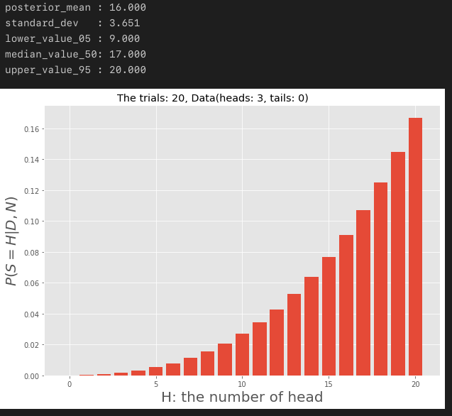
このとき表の出る回数を $S_N$ としたとき、$P(S_N|D)$を求めよ
解答
\[Pr(S_T = H|D) = {}_{N} C_H \int^1_0 \theta^H(1-\theta)^{N-H}P(\theta|D)d\theta\]ともとめることができます. また問題.1より
\[P(\theta|D) = \frac{1}{B(h+1, t+1)}\theta^{h}(1-\theta)^{t}\]なので、
\[\begin{aligned} Pr(S_T = H|D) &= \frac{_{N} C_H}{B(h+1, t+1)} \int^1_0 \theta^{H+h}(1-\theta)^{N-H+t}d\theta\\[8pt] &= {}_{N} C_H\frac{B(H+h+1, N-H+t+1)}{B(h+1, t+1)} \end{aligned}\]解答終了
1
2
3
4
5
6
7
8
9
10
11
12
13
14
15
16
17
18
19
def plot_extrapolate(N_trials, heads, tails, alpha=1, beta=1, ax = None):
    x = np.arange(0, N_trials + 1)
    y = special.comb(N_trials, x) \
        * special.beta(x + heads + alpha,N_trials - x + tails + beta)\
        / special.beta(heads + alpha,tails + beta)

    if ax == None:
      fig, ax = plt.subplots(figsize = (10, 7))

    ax.bar(x, y)
    ax.set_xlabel("H: the number of head", fontsize=20)
    ax.set_ylabel(r"$P(S = H|D, N)$", fontsize=20)
    ax.set_title("The trials: {}, Data(heads: {}, tails: {}) \
                 ".format(N_trials, heads, tails));

    return x, y

x, y = plot_extrapolate(N_trials = 20 , heads = 3, tails = 0)
summary_stats(x, y)
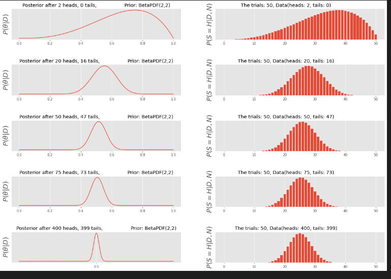
観測Dataを変更してシミュレーション(alpha = 1, beta = 1)
1
2
3
4
5
6
7
8
9
10
11
12
13
14
15
flips = [(2, 0), (20, 16), (50, 47), (75, 73), (400, 399)]
fig, axes = plt.subplots(len(flips), 2, figsize = (20, 14))

for i, flip in enumerate(flips):
    plot_posterior(heads=flip[0], tails=flip[1], alpha=1, beta=1, ax=axes[i,0])
    axes[i,0].set_yticks([])
    plot_extrapolate(N_trials = 50, heads = flip[0], tails = flip[1], ax = axes[i,1])

fig.subplots_adjust(hspace=0.8)
for ax in axes:
    ax[0].set_yticks([])
    ax[1].set_yticks([])
    ax[0].set_xlabel("")
    ax[1].set_xlabel("")
axes[4,0].set_xticks([0.5]);

alpha = 2, beta = 2の場合のシミュレーション
1
2
3
4
5
6
7
8
9
10
11
12
13
14
15
flips = [(2, 0), (20, 16), (50, 47), (75, 73), (400, 399)]
fig, axes = plt.subplots(len(flips), 2, figsize = (20, 14))

for i, flip in enumerate(flips):
    plot_posterior(heads=flip[0], tails=flip[1], alpha=2, beta=2, ax=axes[i,0])
    axes[i,0].set_yticks([])
    plot_extrapolate(N_trials = 50, heads = flip[0], tails = flip[1], alpha=2, beta=2, ax = axes[i,1])

fig.subplots_adjust(hspace=0.8)
for ax in axes:
    ax[0].set_yticks([])
    ax[1].set_yticks([])
    ax[0].set_xlabel("")
    ax[1].set_xlabel("")
axes[4,0].set_xticks([0.5]);
Refereneces
(注意:GitHub Accountが必要となります)