目的
- プレミアリーグ(Man Utd)の試合結果を使って, サッカーの得点分布とポワソン分布の適合度を確認するものです
- この分析において結果的には結構Fitしますが, たまたまだと思ってます.
- アーセナルやシティ, 川崎Fといった攻撃的チームの得点分布はポワソンじゃ説明できない感じです
Table of Contents
Dependency
Python version
- Python 3.9.x
Library
1
2
3
4
5
6
import numpy as np
import pandas as pd
import matplotlib.pyplot as plt
from scipy import stats
from scipy.optimize import minimize
import math
19-20シーズンのMan Utdの得点力分析
READ Data
このMan Utd English Premier League 2019/20 fixture and resultsというサイトではプレミアリーグの各シーズン及び各チームの試合結果が保存されています. ここで抽出にあたってのTipsとして、上記サイトのURLの構造は
1
https://fixturedownload.com/results/epl-<シーズン>/<team名>
となっています. この構造に注意して今回は
| parameter | parameter value | 意味 |
|---|---|---|
| team名 | man-utd |
Man Utd, すべて小文字、スペースはハイフンとなる |
| シーズン | 2019 |
2019-2020シーズン |
という軸でデータを抽出します.
Python
1
2
3
4
5
6
target_team = 'man-utd'
TARGET_TEAMNAME = target_team.replace('-', ' ').title()
URL_PATH = 'https://fixturedownload.com/results/epl-2019/'+target_team

df = pd.read_html(URL_PATH, flavor="bs4")[0]
df.head()
出力結果は
| Round Number | Date | Location | Home Team | Away Team | Result | |
|---|---|---|---|---|---|---|
| 0 | 1 | 11/08/2019 16:30 | Old Trafford | Man Utd | Chelsea | 4 - 0 |
| 1 | 2 | 19/08/2019 20:00 | Molineux Stadium | Wolves | Man Utd | 1 - 1 |
| 2 | 3 | 24/08/2019 15:00 | Old Trafford | Man Utd | Crystal Palace | 1 - 2 |
| 3 | 4 | 31/08/2019 12:30 | St. Mary\'s Stadium | Southampton | Man Utd | 1 - 1 |
| 4 | 5 | 14/09/2019 15:00 | Old Trafford | Man Utd | Leicester | 1 - 0 |
前処理
どのような処理が必要か?
read_htmlで呼び出されたDataFrameは試合結果がResultカラムに格納されていますが、以下の問題点があります:
Home - Awayの順番でスコアが格納されているので、試合ごとのAwayチーム(or Homeチーム)を参照して、どちらの数値がMan Utdの数値か判断する必要あり- 今回はポワソン回帰したいので、スコアが現状では文字列になっているが、それをIntegerに修正する必要があり
Pythonで前処理用関数の定義
1
2
3
4
5
6
7
8
9
10
11
12
13
14
15
16
def extract_score(data, target_team, score_col = 'Result'):
    score_list = data[score_col].str.split(r'\s-\s', expand= True)
    score_list.columns = ['home_score', 'away_score']
    score_list = score_list.astype({'home_score': 'int64', 'away_score': 'int64'})

    df = pd.concat([data, score_list], axis = 1)
    df['score_per_game'] = np.where(df['Home Team'] == target_team, df['home_score'], df['away_score'])
    df['loss_per_game'] = np.where(df['Away Team'] == target_team, df['home_score'], df['away_score'])

    return df

def extract_opponent_team(data, target_team, columns = ['Home Team', 'Away Team'], export_column = 'opponent_team'):
    data[export_column] = data[columns[0]] + data[columns[1]]
    data[export_column] = data[export_column].replace(target_team, '', regex=True)

    return data
Pythonで前処理実行
1
2
3
df_transformed = extract_opponent_team(data = df, target_team = TARGET_TEAMNAME)
df_transformed = extract_score(df_transformed, target_team = TARGET_TEAMNAME)
df_transformed.head()
出力結果は
| Round Number | Date | Location | Home Team | Away Team | Result | opponent_team | home_score | away_score | score_per_game | loss_per_game | |
|---|---|---|---|---|---|---|---|---|---|---|---|
| 0 | 1 | 11/08/2019 16:30 | Old Trafford | Man Utd | Chelsea | 4 - 0 | Chelsea | 4 | 0 | 4 | 0 |
| 1 | 2 | 19/08/2019 20:00 | Molineux Stadium | Wolves | Man Utd | 1 - 1 | Wolves | 1 | 1 | 1 | 1 |
| 2 | 3 | 24/08/2019 15:00 | Old Trafford | Man Utd | Crystal Palace | 1 - 2 | Crystal Palace | 1 | 2 | 1 | 2 |
| 3 | 4 | 31/08/2019 12:30 | St. Mary\'s Stadium | Southampton | Man Utd | 1 - 1 | Southampton | 1 | 1 | 1 | 1 |
| 4 | 5 | 14/09/2019 15:00 | Old Trafford | Man Utd | Leicester | 1 - 0 | Leicester | 1 | 0 | 1 | 0 |
Summary statistics
| score_per_game | loss_per_game | |
|---|---|---|
| count | 38.00 | 38.0 0 |
| mean | 1.73 | 0.94 |
| std | 1.34 | 0.83 |
| var | 1.82 | 0.69 |
| min | 0.00 | 0.00 |
| 25% | 1.00 | 0.00 |
| 50% | 2.00 | 1.00 |
| 75% | 3.00 | 1.75 |
| max | 5.00 | 3.00 |
得点分布をヒストグラムで確かめてみる
1
2
3
4
plt.subplots(figsize=(12, 8))
plt.bar(*np.unique(df_transformed['score_per_game'], return_counts=True))
plt.xlabel('Score per game in 2019-20')
plt.ylabel('Count');

Poisson Fitting
確率変数$X$を一試合あたりの得点数とし, かつポワソン分布に従うとすると確率関数は以下のように書けます:
\[\begin{align*} p(X=x) = \frac{\lambda^x}{x!}\exp(-\lambda) \end{align*}\]$\hat\lambda$は標本平均で推定できるのでFittingの程度を確認すると以下のようになります:
1
2
3
4
5
6
7
8
9
10
11
12
13
14
15
16
17
18
## generating data
N = len(df_transformed['score_per_game'])
x_range = np.arange(0, max(df_transformed['score_per_game'])+2)


## poisson object
observed_lambda = np.mean(df_transformed['score_per_game'])
observed_var = np.var(df_transformed['score_per_game'], ddof=1)
poisson_rv = stats.poisson(observed_lambda)

## plot
fig, ax = plt.subplots(1, 1,figsize=(10, 7))
ax.bar(*np.unique(df_transformed['score_per_game'], return_counts=True), alpha = 0.5)
ax.plot(x_range, poisson_rv.pmf(x_range)*N, label = 'theoretical pmf')
ax.set_xlabel('outcome')
ax.set_ylabel('Frequency')
ax.set_title('the observed $\lambda$: {:.2f}, the data variance:{:.2f}'.format(observed_lambda, observed_var))
plt.legend();
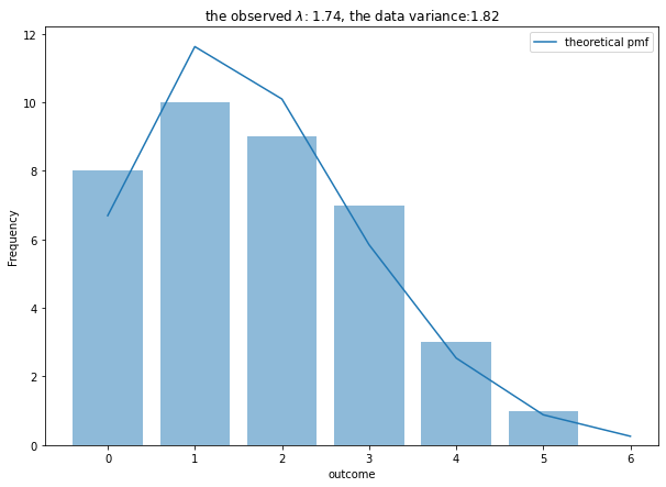
- Fittingはそんなに悪くないがscoreがゼロのところが理論頻度より実現地のほうが多くZIPモデルで回帰してもいいとかも
- 上位チームと戦うときと下位チームで戦うときで戦型を変えてると仮定すると得点は2つ以上の分布の混合分布かもしれない
推定量$\hat\lambda$についてのワルド型信頼区間の計算
推定量$\hat\lambda$の95%信頼区間, $CI$, を簡易的に表現すると以下のようになります
\[CI = \left(\hat\lambda - 1.96 \sqrt{\frac{\hat\lambda}{N}}, \hat\lambda + 1.96 \sqrt{\frac{\hat\lambda}{N}}\right)\]Intuitionとしては, 1試合ごとの得点数を表す確率変数$X_i$, (なお$i$は試合indexを示す), を考えた時, $\hat\lambda$は次のように計算されます:
\[\hat\lambda =\frac{1}{N}\sum_{i}^N X_i\]このとき, $X_i$はパラメーター$\lambda$のポワソン分布に独立に従うと仮定すると
\(\begin{align*} \mathbb E[\hat\lambda] &= \sum_{i}^N\frac{\mathbb E[X_i]}{N} = \lambda\\ V(\hat\lambda) &= \frac{1}{N^2}\sum_{i}^N V[X_i] = \frac{\lambda}{N} \end{align*}\)
従って, $\lambda$を推定量と置き換えて,簡易的に計算すると
\[CI = \left(\hat\lambda - 1.96 \sqrt{\frac{\hat\lambda}{N}}, \hat\lambda + 1.96 \sqrt{\frac{\hat\lambda}{N}}\right)\]が導出されます.
ZIP Fitting
- Appendix: ZIP推定量のクラスで作ったPython Classを用いてZIP paramters $(\lambda, w)$を推定します
1
2
3
zip_mle = ZeroInflatedPoissonRegression(data=df_transformed['score_per_game'])
zip_result = zip_mle.fit()
print(zip_result)
Then,
Optimization terminated successfully.
         Current function value: 62.424527
         Iterations: 36
         Function evaluations: 70
 final_simplex: (array([[1.85621155, 0.06431309],
       [1.85626758, 0.06431888],
       [1.85628597, 0.0643349 ]]), array([62.42452735, 62.42452736, 62.42452738]))
           fun: 62.4245273467983
       message: 'Optimization terminated successfully.'
          nfev: 70
           nit: 36
        status: 0
       success: True
             x: array([1.85621155, 0.06431309])
ZIPパラメータに基づくFittingと可視化
1
2
3
4
5
6
7
8
9
10
11
## poisson object
observed_lambda, zip_w = zip_result.x

## plot
fig, ax = plt.subplots(1, 1,figsize=(10, 7))
ax.bar(*np.unique(df_transformed['score_per_game'], return_counts=True), alpha = 0.5)
ax.plot(x_range, ZeroInflatedPoissonRegression.zip_pmf(x_range, theta = [observed_lambda, zip_w])*N, label = 'theoretical pmf')
ax.set_xlabel('outcome')
ax.set_ylabel('Frequency')
ax.set_title('the zip $\lambda$: {:.2f}, the zip w:{:.2f}, the data variance:{:.2f}'.format(observed_lambda, zip_w, observed_var))
plt.legend();

- 当たり前だけど、普通のポワソン分布で回帰したときよりもFitは上昇する(パラメータ増えているため)
- plotによって可視化したFitをみると、ZIPのあてはまりのよさを見ることができる
Appendix: ZIP推定量のクラス
くわしくは「Ryo’s Tech Blog>統計検定:ポワソン分布と条件付き分布」を読んでください.
1
2
3
4
5
6
7
8
9
10
11
12
13
14
15
16
17
18
19
20
21
22
23
24
25
26
27
28
29
30
31
32
33
34
35
36
37
38
39
40
41
42
43
44
45
46
47
48
49
50
51
52
53
54
55
56
57
58
59
60
61
62
63
64
65
66
67
68
69
70
class ZeroInflatedPoissonRegression:

    def __init__(self, data):
        self.data = data
        self.init_value = None

    @staticmethod
    def zip_pmf(x, theta):
        vec_factorial = np.vectorize(math.factorial)
        return (theta[1] + (1 - theta[1])*np.exp(-theta[0]))**np.where(x > 0, 0, 1) * ((1 - theta[1]) * np.exp(-theta[0]) * theta[0]**x / vec_factorial(x)) **np.where(x > 0, 1, 0)

    @staticmethod
    def em_update(x, theta):
        next_theta_1 = (len(x[x < 1]) - len(x) * np.exp(-theta[0]))/ (1 - np.exp(-theta[0]))
        next_theta_0 = np.sum(x)/(len(x) - next_theta_1)

        return [next_theta_0, next_theta_1]

    def estimate_conditional_poisson(self):
        lambert_w = np.mean(self.data[self.data > 0])
        estimated_lambda = lambertw(-lambert_w/np.exp(lambert_w), 0) + lambert_w

        return estimated_lambda.real

    def method_of_moment(self):
        sample_mean = np.mean(self.data)
        sample_second_moment = np.mean(self.data**2)

        theta_moment = [sample_second_moment / sample_mean - 1, 1 - sample_mean **2 / (sample_second_moment - sample_mean)]
        return theta_moment

    def neg_loglike(self, theta, _data, normalize = False):
        if normalize:
            theta = theta[0], theta[1]/len(_data)

        return np.sum(np.log(self.zip_pmf(x = _data, theta = theta)))

    def fit(self):
        f = lambda theta: -self.neg_loglike(theta = theta, _data = self.data)
        self.init_value = self.method_of_moment()

        return minimize(fun = f, x0=self.init_value, method = 'Nelder-Mead', options={'disp': True})

    def em_fit(self, eps = 1e-10):
        lambda_t = self.estimate_conditional_poisson()
        m_t = len(self.data[self.data < 1])
        theta = [lambda_t, m_t]
        next_theta = self.em_update(self.data, theta)

        while abs(self.neg_loglike(theta = next_theta, _data = self.data, normalize=True) - self.neg_loglike(theta = theta, _data = self.data, normalize=True)) > eps:
            theta = next_theta
            next_theta = self.em_update(self.data, theta)

        next_theta[1] = next_theta[1]/len(self.data)

        return next_theta


## Generating Data
#data = np.repeat(np.arange(0, 7), np.array([22, 23, 26, 18, 6, 4, 1]))
#
## Create the instance
#poisson_mle = ZeroInflatedPoissonRegression(data=data)
#
## fit
#res_mle = poisson_mle.fit().x
#res_em = poisson_mle.em_fit()
#res_mom = poisson_mle.method_of_moment()
#
#print(res_mle, res_em, res_mom)
References
統計検定過去問
- 2012年11月統計検定1級 > 応用数理(共通分野)問2
(注意:GitHub Accountが必要となります)