Table of Contents
問題:Latent variableに依存したパラメーターの推定
Problem
とある地域でポケルスが流行ってるとします. 長年の研究によりポケモン$i$がポケルスに罹患するかしないかは$X_i\in \mathrm R$という確率変数に依存することがわかっており、 ポケモン$i$がポケルスに罹患するかしないかを表した確率変数を$Z_i$とすると
\[Z_i = \begin{cases} 1 & X_i \leq c\\ 0 & \text{ otherwise} \end{cases}\]というメカニズムが知られています. ただ$c$の基準はまだわかっていないとします. $c$の水準を推定するため、とある研究者が地域からランダムにポケモンを無作為に$N$匹抽出し、 罹患数を調べたところ$k$匹がポケルスに罹患しており、その罹患率を$\hat p$と推定しました. ただ調査の不備により$X_i$を調査することはできませんでした = Dataがない. ただ、$X_i$は独立に同じ分布に従っているというとことは過去の研究の蓄積ですでに判明しています.
この状況のもとで$c$を推定したとき以下の設問を考えたいとします
- $\hat p$の推定方法を述べよ
- $\hat p$の漸近分布を述べよ
- $F(\cdot)$をcdfとしたとき$F(X_i) = 1/1 + \exp(-x)$の場合の$c$のstandard deviation
- $X_i\sim N(0, 1)$のときの$c$のstandard deviation
なお、$\hat p$のstandard errorは以下の式で近似できるとする
\[\text{s.e}(\hat p) = \sqrt{\frac{\hat p (1 - \hat p)}{n}}\](1) $\hat p$の推定方法を述べよ
$Z_i$はベルヌーイ試行とみなせるので、モーメント法ならば
\[\mu_Z = (p\exp(0) + 1- p)p = p\]従って、$\mu_Z = \bar Z$と標本対応すると
\[\hat p = \frac{\sum Z_i}{N}=\frac{k}{N}\]最尤法ならば
\[\begin{align*} L(p|Z) &= \prod p^{Z_i}(1 - p)^{Z_i}\\[8pt] \Rightarrow & \log L(p|Z) = \sum Z_i \log p + (1 - Z_i) \log (1 - p)\\[8pt] \Rightarrow & \frac{\partial \log L(p|Z)}{\partial p} = \frac{k}{p} - \frac{N -k}{1-p} \quad\quad\tag{1.1} \end{align*}\](1.1)が0となるような$p$を計算すると
\[\hat p = \frac{k}{N}\](2) $\hat p$の漸近分布を述べよ
確率変数$k$は二項分布$Bin(p, N)$に従っているとみなせるので, その期待値が$Np$, 分散が$Np(1-p)$に留意すると
\[\hat p = \frac{k}{N}\sim \left(p, \frac{p(1-p)}{N}\right)\]Ryo’s Tech Blog > 二項分布に従う確率変数の正規分布近似より、$N\to\infty$のとき
\[\frac{k - Np}{\sqrt{Np(1-p)}}\sim N(0, 1)\]なので、
\[\begin{align*} &\frac{k/N - p}{\sqrt{p(1-p)/N}}\sim N(0, 1)\\[8pt] &\Rightarrow \hat p \sim N\left(p, \frac{p(1-p)}{N}\right) \end{align*}\](3) $F(X_i) = 1/(1 + \exp(-x))$の場合の$c$のstandard deviation
$N$が十分大きい時$\hat p$は$p$にほとんど等しいと考えることができます. そのため、$c$について
\[\hat c = F^{-1}(\hat p)\]と表現した時、Taylor展開より
\[\begin{align*} \hat c &\simeq F^{-1}(p) + (\hat p - p)\frac{\partial F^{-1}(p)}{\partial p} + o(\hat p - p)\\ &\Rightarrow (\hat c - c) \simeq (\hat p - p)\frac{\partial F^{-1}(p)}{\partial p} + o(\hat p - p) \end{align*}\]従って、
\[\begin{align*} \text{s.e}(\hat c) &\simeq \text{s.e}(\hat p)\frac{\partial F^{-1}(p)}{\partial p}\\ &= \frac{\text{s.e}(\hat p)}{F'(F^{-1}(p))} \end{align*}\]つまり、$\text{s.e}(\hat c)$はpを$\hat p$で標本対応させて推定すれば良いことがわかります.
\[F'(x) = \frac{\exp(-x)}{(1 + \exp(-x))^2}\]及び, $x < 1$の範囲において
\[F^{-1}(x) = -\log\left(\frac{1}{x} - 1 \right)\]よって、
\[\text{s.e}(\hat c) = \frac{1}{\sqrt{\hat p (1 - \hat p)N}}\](4) $X_i\sim N(0, 1)$の場合の$c$のstandard deviation
(3)と同様に
\[F^{-1}(\hat p) = z_{p}\]とおくと、
\[\text{s.e}(\hat c) = \exp\left(\frac{z_p^2}{2}\right)\sqrt{2\pi \hat p(1 - \hat p)/N}\]PythonでSimulation
- ソースコードはこちら: Google Colab
推定量のクラス
1
2
3
4
5
6
7
8
9
10
11
12
13
14
15
16
17
18
19
20
21
22
23
24
25
26
27
28
29
30
31
32
33
34
35
36
37
38
39
40
41
42
43
44
45
46
47
48
49
50
51
52
53
54
55
56
57
58
59
60
61
62
63
64
65
66
import numpy as np
from scipy.stats import norm
from scipy.stats import logistic
import matplotlib.pyplot as plt

class pokerus_simulator:

    def __init__(self, sample_size, c, population_distirubution, iter_cnt):
        """
        Args
            sample_size:
                検査のポケモンの数

            c:
                ポケルス感染のthreshold

            population_distirubution:
                ポケルス感染に関連する確率変数の分布
                logisticと指定した場合はロジスティク分布、それ以外は標準正規分布となる

            iter_cnt:
                シミュレーション回数

        """
        self.sample_size = sample_size
        self.c = c
        self.iter_cnt = iter_cnt
        self.data = None
        self.population_distirubution = population_distirubution

    def data_generator(self):
        if self.population_distirubution == 'logistic':
            self.data = logistic.rvs(size=self.sample_size)
        else:
            self.data = norm.rvs(size=self.sample_size)

        self.data = np.where(self.data<self.c, 1, 0)

    def estimate_c(self):
        p_hat = sum(self.data)/self.sample_size
        standard_error_p = np.sqrt(p_hat * (1 - p_hat)/self.sample_size)

        if self.population_distirubution == 'logistic':
            c_hat = -np.log(1/p_hat - 1)
            standard_error_c = 1/np.sqrt(p_hat*(1 - p_hat) * self.sample_size)

        else:
            c_hat = norm.ppf(p_hat)
            standard_error_c = np.exp(c_hat**2/2)*np.sqrt(2*np.pi)*standard_error_p

        return c_hat, standard_error_c, p_hat

    def simulation(self):
        p_hat_array = []
        c_hat_array = []
        c_hat_se_array = []

        for cnt in range(self.iter_cnt):
            self.data_generator()
            c_hat, c_se, p_hat = self.estimate_c()

            p_hat_array.append(p_hat)
            c_hat_array.append(c_hat)
            c_hat_se_array.append(c_se)

        return c_hat_array, c_hat_se_array, p_hat_array
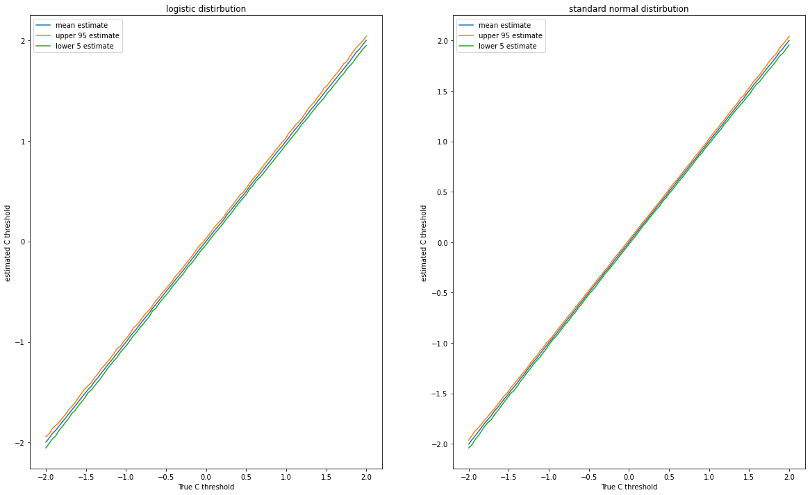
Visulization
1
2
3
4
5
6
7
8
9
10
11
12
13
14
15
16
17
18
19
20
21
22
23
24
25
26
27
28
29
30
31
32
33
34
35
36
37
38
39
40
41
42
43
44
N = 10000
C = np.linspace(-2, 2, 100)
ITER_CNT = 100

fig, ax= plt.subplots(1, 2, figsize = (20, 12))


c_hat_list = []
c_hat_upper = []
c_hat_lower = []

for i in C:
    simulation_batch = pokerus_simulator(sample_size = N, c = i, population_distirubution = 'logistic', iter_cnt = ITER_CNT)
    c_hat, c_se, p_hat = simulation_batch.simulation()
    c_hat_list.append(np.mean(c_hat))
    c_hat_upper.append(np.quantile(c_hat, 0.95))
    c_hat_lower.append(np.quantile(c_hat, 0.05))

ax[0].plot(C, c_hat_list, label = 'mean estimate')
ax[0].plot(C, c_hat_upper, label = 'upper 95 estimate')
ax[0].plot(C, c_hat_lower, label = 'lower 5 estimate')

ax[0].set_xlabel('True C threshold')
ax[0].set_ylabel('estimated C threshold')
ax[0].set_title('logistic distirbution')
ax[0].legend();

c_hat_list = []
c_hat_upper = []
c_hat_lower = []
for i in C:
    simulation_batch = pokerus_simulator(sample_size = N, c = i, population_distirubution = 'normal', iter_cnt = ITER_CNT)
    c_hat, c_se, p_hat = simulation_batch.simulation()
    c_hat_list.append(np.mean(c_hat))
    c_hat_upper.append(np.quantile(c_hat, 0.95))
    c_hat_lower.append(np.quantile(c_hat, 0.05))

ax[1].plot(C, c_hat_list, label = 'mean estimate')
ax[1].plot(C, c_hat_upper, label = 'upper 95 estimate')
ax[1].plot(C, c_hat_lower, label = 'lower 5 estimate')
ax[1].set_xlabel('True C threshold')
ax[1].set_ylabel('estimated C threshold')
ax[1].set_title('standard normal distirbution')
ax[1].legend();
References
(注意:GitHub Accountが必要となります)