Table of Contents
- 問題意識
- Permutation Test
- Paired Permutation Test
- 相関係数とPermutation Test
- Regression CoefficientとPermutation Test
- References
問題意識
2つ以上の分布の同一性を確かめる手法の一つとして, 「ウェルチのT検定」はよく用いられてます(例: ABテストとかの文脈). しかし, 母集団分布に形状に応じてはhighly skewedなどの理由で「mean」を母集団を特徴づける統計量として用いることが適切ではないとか, T分布に従うという仮説に下で検定することが少し無理がある場合など, 分布形の仮定無しで検定したいというニーズがあります.
このノートではノンパラメトリック検定の1つ, Permutation Testを簡単にまとめます.
p-valueの注意点
Permutation Testにおいてp-valueという言葉が出てきますが意味としては
- p-value: Given that the null hypothesis is true, the p-value is the probability that we measure a statistic at least as extreme as the observed result
つまり, いわゆるthe null hypothesisが正しい確率ではなくて, the null hypothesisが正しいと仮定したときに観測された統計量がどれだけレアなのかを意味するに過ぎません. (the null hypothesisとデータがどれだけ整合的か?と解釈することは良いと思いますが)
Permutation Test
Permutation Test(並べ替え検定)は2つのグループを比較するノンパラメトリック検定の一つです. 帰無仮説の下では2つのグループが同一分布に従う, 対立仮説は2つのグループが異なる分布に従うとします.
Permutation Test Mechanics
- 観察データに基づき, 2つにグループ間の差の統計量(例: mean, medianの差)を計算する
- データについてAll possible permutationを実行し, 上記と同じグループ間統計量をそれぞれ計算する
- (1)について計算した統計量が(2)の統計量と照らし合わせて, どれくらい極端であったか計算する(いわゆるp-valueの計算)
- $t_0$: 観察されたグループ間統計量(例: mean, medianの差)
- $n, m$はそれぞれのグループのサイズ
- $n, m$のサイズに対して, permutationすべてを評価する計算量が$O((n+m)!)$であることに留意
PythonでのPermutation Test実行
observationsをtreatとcontrolの2つのグループに分け, なにかしらの値を測定したとします.
この測定した値がtreatとcontrolで異なる分布になるのか否か検定する場合の例を紹介します.
1
2
3
4
5
6
7
8
9
10
11
12
13
14
15
import numpy as np
from scipy.stats import permutation_test

treat = np.array([114, 203, 217, 254, 256, 284, 296])
control  = np.array([4, 7, 24, 25, 48, 71, 294])

def statistic(x, y, axis):
    return np.median(x, axis) - np.median(y, axis)

res = permutation_test((treat, control), statistic, vectorized=True,
                       n_resamples=np.inf, alternative='greater') ##n_samples=np.infはexact test

res_median, res_pvalue, res_null = res.statistic, res.pvalue, res.null_distribution
print(res_pvalue)
>>> 0.017482517482517484
なお, ここでのp-valueは以下の計算と一致します:
1
2
np.count_nonzero(res_null >= res_median - max(1e-14, res_median * 1e-14)) / len(res_null)
>>> 0.017482517482517484
permutation_testでは統計量についてmax(1e-14, abs(r)*1e-14)の範囲内に該当するnull distributionもカウントしているとのこと- scipy documentでは「This method of comparison is expected to be accurate in most practical situations」と一応コメントしている
Median Differenceの95% CIの計算方法
2つの分布の検定だけでなくConfidence Intervalによる不確実性(統計量の分散)も確認したいケースは多々あります. ここで紹介するやり方はシンプルにBootstrap法に基づいて計算する方法となります.
1
2
3
4
5
6
7
8
9
10
11
12
13
14
15
def two_sample_bootstrap(x, y, statistic, size, percentile):
    boot_res = []
    for i in range(size):
        tmp_x = np.random.choice(x, len(x), replace=True) ## x[np.random.randint(0, len(x), len(x))]の方が早い
        tmp_y = np.random.choice(y, len(y), replace=True)
        tmp_stats = statistic(tmp_x, tmp_y)
        boot_res.append(tmp_stats)

    return np.quantile(boot_res, [1 - percentile, percentile])

def statistic_median(x, y):
    return np.median(x) - np.median(y)

two_sample_bootstrap(treat, control, statistic_median, 100000, 0.975)
>>> (132, 260) ### Rのsimpleboot, bootと結果は一致
Paired Permutation Test
細胞にとある処置をするとその細胞の成長スピードが上昇するという仮説をいま持っているとします. これを検証するRCTを実施するため, 10個の細胞をどこかから取得してきて, それぞれに対してクローンを作成します(同じ細胞を元に作成されたペアの作成).
それぞれのペアについて, 独立にコインを投げてtreated, controlの分類をし, 一定時間後にそれらの成長スピードを観測したとします, = $(x_i, y_i)$を観測. コインの出るパターンは $2^{100}$通り存在しますが, そのうちの一つが実現したと理解できます.
観測したデータに基づき, 平均やMedianの差といった統計量 $T_{obs}$を計算し, それをテストしたいというのがモチベーションです.
\[(x_1, y_1), \cdots, (x_{100}, y_{100}) \to T_{obs}\]Paired Permutation Testは, the null hypothesisがどちらも同一分布に従っているという仮説(具体的には平均やMedianが同じ)の下ならば, 実現値である$(x_i, y_i)$を入れ替えて $T$を新たに計算してもその$T$に対して$T_{obs}$は極端な値にならないはずだし, 入れ替えパターン$2^{100}$通りについても同様に計算し, simulation dataについて得られた$2^{100}$通りの$T$に対しても, $T_{obs}$はそんなに極端にはならないだろうという形で実行するノンパラ検定です.
| observed pair | simulated pair(例) |
|---|---|
| [3.67, 2.11] | [3.67, 2.11] |
| [1.72, 1.79] | [1.79, 1.72] |
| [3.46, 2.71] | [2.71, 3.46] |
| [2.60, 1.89] | [2.60, 1.89] |
Scipyでの実行方法
1
2
3
4
5
6
7
8
9
10
11
12
13
14
15
import numpy as np
from scipy.stats import permutation_test

def statistic(x, y):
    return np.median(x) - np.median(y)

x = [3.67, 1.72, 3.46, 2.60, 2.03, 2.10, 3.01]
y = [2.11, 1.79, 2.71, 1.89, 1.69, 1.71, 2.01]

res_sci = permutation_test((x, y), statistic, vectorized=False,
                       n_resamples=np.inf,
                       permutation_type='samples',
                       alternative='two-sided')
print(res_sci.pvalue)
>>> 0.0625
permutation_type='samples'にすることを忘れずに
なお, approximateに実行する場合は基本的には以下のコードと同じ挙動をします
(上の例におけるpermutation_test=整数値でも大丈夫です)
1
2
3
4
5
6
7
8
9
10
11
12
13
14
15
16
17
18
19
20
21
x = [3.67, 1.72, 3.46, 2.60, 2.03, 2.10, 3.01]
y = [2.11, 1.79, 2.71, 1.89, 1.69, 1.71, 2.01]
z = np.array([x, y])

def two_sample_permutation(z, statistic, size):
    boot_res = []
    z_len = z.shape[1]
    array_idx = np.arange(0, z_len)
    for i in range(size):
        flip_coin = np.random.randint(0, 2, z_len)
        tmp_x = z[flip_coin, array_idx]
        tmp_y = z[1 - flip_coin, array_idx]
        tmp_stats = statistic(tmp_x, tmp_y)
        boot_res.append(tmp_stats)

    return boot_res

res = two_sample_permutation(z=z, statistic=statistic, size=1000)
obs = np.median(y) - np.median(x)
np.count_nonzero(np.abs(res) >= np.abs(obs)) / len(res)
>>> 0.062
相関係数とPermutation Test
とある変数の組 $(X, Y)$ の関係性についてリサーチしたいとして, その取っ掛かりとして$(X, Y)$の相関係数について分析するとします. $(X, Y)$が互いに独立(無相関)だとしても, 相関係数が0と異なる値が出る可能性がある中, 手元のデータが無相関であるというthe null hypothesisとどれだけ整合的か/不整合的か評価する際にもPermutation Testは利用できます.
ただし, 異なる確率変数$(X, Y)$ の関係性について検定したいので, 普通のPermutation Testとは異なり $X = (x_1, x_2, \cdots, x_n)$と$Y = (y_1, y_2, \cdots, y_n)$の中で順番入れ替えを実施します. もしthe null hypothesisが正しいならば$X$と$Y$のそれぞれの中で順番を入れ替えたとしても手元のデータから得られた統計量とそんなに差がないはずだというのがモチベーションです.
手順
- 検定統計量の設定, 今回は $\rho(X, Y)$
- the null hypothesisの設定, $H_0: \rho(X, Y)=0$
- the alternative hypothesisの設定, $H_1: \rho(X, Y)>0$
- Permutation Setの構築: $X$と$Y$のそれぞれの中で順番をランダムに入れ替える
Pythonでの実行例
QuantEconより為替レート調整済み一人あたりGDPと資産保護index についてのデータを用いて, これら2変数の相関関係を確認してみます.
1
2
3
4
5
6
7
8
df = pd.read_stata('https://github.com/QuantEcon/lecture-python/blob/master/source/_static/lecture_specific/ols/maketable1.dta?raw=true')
df = df.dropna()
y, x = df['logpgp95'].values, df['avexpr'].values

plt.scatter(x, y)
plt.title('size = {}, correlation = {:.2}'.format(len(x), pearsonr(x, y)[0]))
plt.xlabel('avexpr')
plt.ylabel('logpgp95');

欠損値を含んだレコードを除去したあとにscatter plotで確認してみると資産保護indexが高いほど一人あたりlog GDPが高い傾向にあるこることがわかります. 相関係数を計算すると0.75という値が出力されますが, $H_0: \rho= 0, H_1:\rho >0$, に対してどれくらいレアなものかPermutation Testで以下検定します.
1
2
3
4
5
6
7
8
9
10
11
12
13
14
### Permutation Test
def statistic_r(x, y):
    return pearsonr(x, y)[0]

res = permutation_test((x, y), statistic_r, vectorized=False,
                       permutation_type='pairings',
                       alternative='greater')

### 可視化
count, bins, _ = plt.hist(res.null_distribution, bins=100)
plt.vlines(obs_corr, 0, max(count),
           colors='red', linestyles='dashed'
          )
plt.title('Permuation Test: Corr coef Distirbution: p-value = {}'.format(res.pvalue))
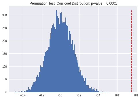
資産保護indexと一人あたりlog GDPが互いに独立(無相関)というthe null hypothesis下ではなかなか見られない相関係数が 手元では得られたということが読み取れます.
Regression CoefficientとPermutation Test
Permutation TestをEconometricsの文脈で用いる際,
- 検定の文脈に置いてPermutation Testと一般的なt-testはどのように異なるのか?
- Permutation Testの検出力はどんなもんなのか?
という観点が気になると思います. 単回帰に関するMonte Carlo Simulationで棄却率をt-testと比較確認してみたいと思います.
Monte Carlo Simulation設定
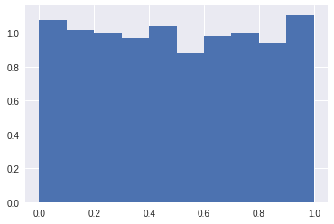
\[y_i = \beta_1 + \beta_2 x_i + \epsilon_i; \ \ i = 1, 2, \cdots, N\]という単回帰モデルを考えます. $x_i, \epsilon_i$はそれぞれ独立に$N(0, 1)$に従うとします. ここでは$\beta_1 = 1$に固定, $(\beta_2, N)$をパラメーターとして, simulation回数を1 batch 2000回で棄却率をt-test, perm-testでそれぞれ計算するとします.
error termがhomoskedastic & iid normally distributedなので, t-testの仮定が満たされる状況下となっています. T-testの仮定が正しい中, Perm-testでも似たような棄却率が出てくるのか確認するのが目的です.
Perm testはノンパラ検定なので, iidとかの仮定は必要ですが, homoskedasticityやnot-skewedの仮定がいらないので, もし似通った棄却率を叩き出すならば結構良いなというのが期待値です.
\[\begin{align*} \beta_2 & \in (0, 0.1, 0.2, \cdots, 1)\\ N &\in (15, 30) \end{align*}\]パラメーター空間
Python Code: 実行時間は30 minくらい
1
2
3
4
5
6
7
8
9
10
11
12
13
14
15
16
17
18
19
20
21
22
23
24
25
26
27
28
29
30
31
32
33
34
35
36
37
38
39
40
41
42
43
44
45
46
47
48
49
50
51
52
53
54
55
56
57
58
59
60
61
62
63
64
65
66
67
68
69
70
71
72
73
74
75
76
import statsmodels.api as sm
import itertools
from multiprocessing import Pool
import collections

N = [15, 30]
const = [1]
beta = np.linspace(0, 1, 11)
sig_level = 0.05
nrep = 2000
seed = 42

def flatten(l):
    for el in l:
        if isinstance(el, collections.abc.Iterable) and not isinstance(el, (str, bytes)):
            yield from flatten(el)
        else:
            yield el

def func_dgp(size, const, beta):
    eps = np.random.normal(0, 1, size)
    x = np.random.normal(0, 1, size)
    y = const + x * beta + eps

    return y, x

def compute_ttest(y, X):
    _X = sm.add_constant(X)
    model = sm.OLS(y,_X)
    result = (model.fit()).t_test([0,1])
    return result.effect, result.pvalue

def compute_permtest(y, X):
    def perm_statistics(_y, _X):
        return np.cov(_y, _X, ddof=-1)[0,1]/np.var(_X, ddof=-1)

    res = permutation_test((y, X), perm_statistics, vectorized=False,
                            n_resamples=2000,
                            permutation_type='pairings',
                            alternative='two-sided')

    return res.statistic, res.pvalue


def compute_power_analysis(params):
    record = []
    t_power, p_power = [], []
    for i in range(nrep):
        y, X = func_dgp(*params)
        t_coef, t_pval = compute_ttest(y, X)
        t_power.append(t_pval)
        p_coef, p_pval = compute_permtest(y, X)
        p_power.append(p_pval)

    power_list = [np.mean(np.array(t_power) < sig_level), np.mean(np.array(p_power) < sig_level)]

    params = list(params)
    params.extend(*zip([power_list]))

    record.extend(list(flatten(params)))

    return record

## table
p = Pool(6)
res = p.map(compute_power_analysis, [param for param in list(itertools.product(*[N, const, beta]))])
table_1 = pd.DataFrame(res, columns=['obs_size', 'const', 'beta', 't_test_power', 'perm_test_power'])

## p-value distribution
p = Pool(6)
res_pval_dist =  p.map(compute_power_analysis_pval, [(15, 1, 0, 2000)])
plt.hist(res_pval_dist, bins=np.linspace(0, 1, 11), density=True);

from scipy import stats
stats.kstest(res_pval_dist,stats.norm.cdf)
>>> KstestResult(statistic=0.8413447460685429, pvalue=0.31731050786291415)
Simulation結果
下のテーブルがsimulation結果となります. 棄却率はt-test, Perm-testそれぞれ似通った値となっています. また, $\beta_2=0$の時のp-value distributionを確認すると “reasonably uniform” となっており一応期待された結果となっております 実際に, p-valueヒストグラムを確認すると特定のp-valueが出力されやすいということは確認されなかったと解釈しても良いかもですし, KS testで一様性の検定をしたところ, 棄却はされなかったという結果になっております.
| obs_size | True beta | t-test棄却率 | perm-test棄却率 |
|---|---|---|---|
| 15 | 0.0 | 0.0460 | 0.0505 |
| 15 | 0.1 | 0.0550 | 0.0570 |
| 15 | 0.2 | 0.0975 | 0.0965 |
| 15 | 0.3 | 0.1735 | 0.1700 |
| 15 | 0.4 | 0.2715 | 0.2665 |
| 15 | 0.5 | 0.3965 | 0.3985 |
| 15 | 0.6 | 0.5180 | 0.5115 |
| 15 | 0.7 | 0.6305 | 0.6220 |
| 15 | 0.8 | 0.7420 | 0.7355 |
| 15 | 0.9 | 0.8255 | 0.8190 |
| 15 | 1.0 | 0.8990 | 0.8915 |
| 30 | 0.0 | 0.0485 | 0.0500 |
| 30 | 0.1 | 0.0960 | 0.0945 |
| 30 | 0.2 | 0.1920 | 0.1890 |
| 30 | 0.3 | 0.3360 | 0.3345 |
| 30 | 0.4 | 0.5335 | 0.5305 |
| 30 | 0.5 | 0.7200 | 0.7160 |
| 30 | 0.6 | 0.8500 | 0.8495 |
| 30 | 0.7 | 0.9305 | 0.9290 |
| 30 | 0.8 | 0.9725 | 0.9715 |
| 30 | 0.9 | 0.9905 | 0.9915 |
| 30 | 1.0 | 0.9970 | 0.9975 |
References
- Foundations of Statistics for Data Scientists: With R and Python
- scipy > scipy.stats.permutation_test
- mlxtend > permutation_test: Permutation test for hypothesis testing
- David Garcia, 2021, Permutation Tests
- QuantEcon > 75. Linear Regression in Python
- R bloggers > A Permutation Test Regression Example
(注意:GitHub Accountが必要となります)