マルサスモデル
練習 1 : マルサスの人口論
時刻 \(t\) におけるとある国の人口が \(N(t) > 0\) で表されるとする.マルサスは時刻 \(t\) から \(t+\Delta t\) の人口増分 \(\Delta N = N(t+\Delta) - N(t)\) は
\[ \Delta N = k N(t)\Delta t \qquad (k: \text{constant}) \]
のように \(N, \Delta t\) に比例するとした.ここから以下のように式変形を行い
\[ \frac{\Delta N}{\Delta t} = k N(t) \]
\(\Delta t\to 0\) として次のような微分方程式を得たとします
\[ \frac{dN(t)}{dt} = kN(t) \label{eq-de-01} \]
\((t, N(t))\) が \((0, 1.00 \times 10^8), (1, 1.25 \times 10^8)\) と与えられているとき,\(t = 2\) の人口 \(N(2)\) を推定せよ.
▶ Python Simulation
scipy.integrateパッケージのodeintを用いれば微分方程式を解くことができます.
コード
import numpy as np
from scipy.integrate import odeint
import matplotlib.pyplot as plt
# malthusian growth func
def malthusian_model(y, t, k=np.log(1.25)):
dydt = k * y
return dydt
# init
N_0 = 1.0
# data point
data = (0, 1), (1, 1.25)
# time
t = np.linspace(0, 5, 21)
# solve
n = odeint(malthusian_model, N_0, t)
# plot
plt.plot(t, n)
plt.scatter(*zip(*data), color='red', label='observed data points')
plt.legend()
plt.xlabel("t")
plt.ylabel("$N(t)$")
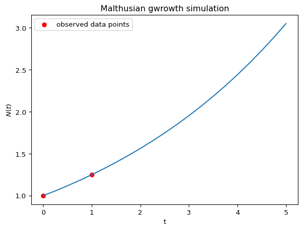
plt.title("Malthusian gwrowth simulation")
plt.show()図 1 をみると \(N(t)\) は指数関数的に増加していることが読み取れます.これは \(k\) の符号に依存しています.
- \(k > 0\): 指数関数的増加
- \(k = 0\): 変化なし
- \(k < 0\): 指数関数的減衰
となります.図示すると以下のようになります
コード
import statsmodels.api as sm

# params
k_args = (-0.2, 0, 0.2)

# solve
for k in k_args:
    n = odeint(malthusian_model, N_0, t, args=(k,))
    plt.plot(t, n, label=f"k={k}")

plt.legend()
plt.xlabel("t")
plt.ylabel("$N(t)$")
plt.title("Malthusian growth simulation with different $k$")
plt.show()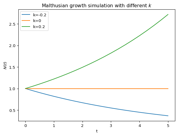
Estimation & Prediction
- \(N(t)\) は 4期間ごとに観測される(=観測されるtは\((0, 1, 2, 4)\))
- 観測される \(N(t)\) にはノイズが乗ってしまっている: \(\epsilon_t \sim N(0, 0.1)\)
という状況ののもと,\((N_0, k)\) を推定し,\(t>4\) の範囲の人口について予測することはできるのか?という問題を考えてみます.
\(\eqref{eq-malthus-solution}\) について対数を取ると
\[ \log N(t) = \log(N_0) + kt \]
となります.つまり,対数変換した変数についての線形モデルとして推定量を考えることができます.観測ノイズ \(\epsilon_t\) を踏まえると,観測される人口を \(\tilde N(t)\) とすると
\[ \begin{align} &\tilde N(t) = N_0\exp(kt) + \epsilon_t\\ &\Rightarrow\log \tilde N(t) = \log (N_0\exp(kt) + \epsilon_t) \end{align} \]
となってしまいますが,近似式として
\[ \log\tilde N(t) = \alpha + \beta t + e_i \]
で推定するとします.\(\epsilon_i\)がhomogeneousとしても\(e_i\)がhomogeneousとは限らないのでheteroskedasticity residual erroを想定して推定します.
コード
import statsmodels.api as sm

np.random.seed(42)

# observation step
STEP = 4

# DGP
actual_n = n.flatten()
observed_n = actual_n[::STEP][:-1] + +np.random.normal(0, 0.1, len(actual_n[::STEP][:-1]))
observed_t = t[::STEP][:-1]
X = sm.add_constant(observed_t)

# fit
model = sm.OLS(np.log(observed_n), X).fit(cov_type="HC0")
estimated_n_0, estimated_k = model.params

# simulation
simulated_n = odeint(malthusian_model, np.exp(estimated_n_0), t, args=(estimated_k,))

# plot
plt.plot(t, simulated_n, label="simulated")
plt.scatter(observed_t, observed_n, color="gray", alpha=0.8, marker='x', label="actual data points")
plt.scatter(t, actual_n, color="red", alpha=0.8, label="actual data points")
plt.legend()
plt.xlabel("t")
plt.ylabel("$N(t)$")
plt.title("Malthusian growth prediction")
plt.axvspan(4.25, t[-1], color='gray', alpha=0.3)
plt.text(4.65, 2.0, "Prediction\nPeriod", ha='center', va='center', fontsize=11, color='black')
plt.show()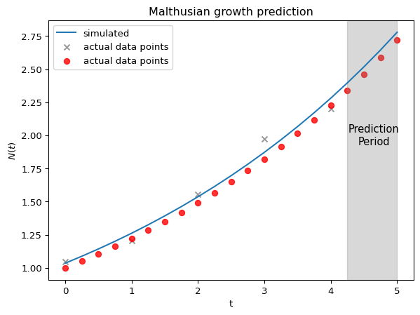
ヴェアフルストの人口論
人口過密の要因を考慮に入れてマルサスモデルを修正したのがヴェアフルストモデルです.
▶ 仮定の設定
- 人口の上限 \(N_\infty\) が存在する
- 現在の人口を \(N(t)\) としたとき,人口増加 \(\Delta N(t)\) は \(N(t)\) と \(\displaystyle 1 - \frac{N(t)}{N_\infty}\) と時間区間 \(\Delta\) に比例する
▶ 問題の定式化
比例定数を \(k\) としたとき
\[ \Delta N(t) = kN(t)\left(1 - \frac{N(t)}{N_\infty}\right)\Delta t \]
\(\Delta t\to 0\) と極限をとると
\[ \frac{dN(t)}{dt} = kN(t)\left(1 - \frac{N(t)}{N_\infty}\right)\label{eq-logistic-model} \]
人口変化は上記のような一階上微分方程式で表せるという形で定式化できました.
▶ モデルを解く
\(\eqref{eq-logistic-model}\) を変形すると
\[ \frac{N_\infty}{N_\infty - N(t)}\frac{dN(t)}{N(t)dt} = k \]
両辺を \(t\) について積分すると
\[ \begin{align} & \int\frac{N_\infty}{N_\infty - N(t)}\frac{dN(t)}{N(t)dt} dt= \int k dt\\ &\Rightarrow \int\left(\frac{1}{N(t)}+\frac{1}{N_\infty - N(t)}\right)dN(t) = \int k dt\\ &\Rightarrow \log N(t) - \log(N_\infty - N(t)) = kt + C\\ &\Rightarrow \log \frac{N(t)}{N_\infty - N(t)} = kt + C \end{align} \]
このとき,\(N(0) = N_0\) と初期条件が与えられたとすると
\[ \exp(C) = \frac{N_0}{N_\infty - N_0} \]
よって,
\[ \frac{N(t)}{N_\infty - N(t)} = \frac{N_0}{N_\infty - N_0}\exp(kt) \]
これを \(N(t)\) についてとくと,
\[ N(t) = \frac{N_\infty}{1 + [(N_\infty/N_0 - 1)]\exp(-kt)} \]
または
\[ \frac{1}{N(t)} = \frac{1}{N_\infty} + \left(\frac{1}{N_0} - \frac{1}{N_\infty}\right)\exp(-kt) \]
▶ 解釈
\(t\to\infty\) のとき,\(\lim_{t\to\infty}\exp(-kt) = 0\) より
\[ \lim_{t\to\infty}N(t) = N_\infty \]
となることがわかります.初期値に応じて \(N_\infty\) へ到達する経路は異なります.仮に \(N_\infty = 12, k=0.2\) として,初期値が \((1, 3, 6, 9, 12, 15)\) と異なる水準で与えられたとします.
コード
from scipy.integrate import solve_ivp


# Define logistic growth model
def logistic_growth(t, N, k=0.2, M=12):
    dydt = k * N * (1 - N / M)
    return dydt

# Set up the grid for the direction field
t_vals = np.linspace(0, 30, 20)  # Time values
P_vals = np.linspace(0, 16, 20)  # Population values
T, P = np.meshgrid(t_vals, P_vals)

# Compute direction field (dP/dt values)
dP_dt = logistic_growth(None, P)

# Normalize arrows for visualization
norm = np.sqrt(1**2 + dP_dt**2)
U = 1 / norm  # Time step is 1 (arbitrary)
V = dP_dt / norm  # Scale arrows properly

# Plot the direction field
plt.figure(figsize=(8, 5))
plt.quiver(T, P, U, V, color="gray", alpha=0.7) # [T, P]: arrow location, [U, V]: arrow direction

# Solve the ODE for different initial conditions
initial_conditions = [1, 3, 6, 9, 12, 15,]
t_span = (0, 30)
t_eval = np.linspace(0, 30, 100)

for P0 in initial_conditions:
    sol = solve_ivp(logistic_growth, t_span, [P0], t_eval=t_eval)
    if sol.success:
        plt.plot(sol.t, sol.y[0], linewidth=2, label=f"P(0)={P0}")
    else:
        raise ValueError("computation failed")

# Labels and title
plt.xlabel("t")
plt.ylabel("P(t)")
plt.title("Logistic Growth Model")
plt.legend()
plt.grid()

# Show the plot
plt.show()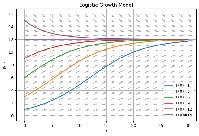
- \(0< N_0 < N_\infty\): はじめの増加は指数関数的だが,ある程度の水準から増加の度合いは減衰していく
- \(N_0 = N_\infty\): 変化なし
- \(N_0 > N_\infty\): \(N_\infty\)に近づく方向で減少していく.減衰の度合いは減衰していく
- \(N_0 = 0\): これも一つの均衡だが,ちょっとしたショックがあるだけで \(N_\infty\) を目指すPathに乗ってしまう(= unstable equilibrium)
▶ Validation
ヴェアフルストモデルが人口動態を表した良いモデルなのか,1820-1930のアメリカの人口データを用いて検証してみます.
コード
import pandas as pd

# Historical population data (year, population in millions)
data = {
    "year": [1820, 1830, 1840, 1850, 1860, 1870, 1880, 1890, 1900, 1910, 1920, 1930, 2000],
    "us_population_million": [9.6, 12.9, 17.1, 23.2, 31.4, 38.6, 50.2, 62.9, 76.0, 92.0, 106.5, 123.2, 282.2]
}

# Create DataFrame
df = pd.DataFrame(data)

# Display table
df| year | us_population_million | |
|---|---|---|
| 0 | 1820 | 9.6 |
| 1 | 1830 | 12.9 |
| 2 | 1840 | 17.1 |
| 3 | 1850 | 23.2 |
| 4 | 1860 | 31.4 |
| 5 | 1870 | 38.6 |
| 6 | 1880 | 50.2 |
| 7 | 1890 | 62.9 |
| 8 | 1900 | 76.0 |
| 9 | 1910 | 92.0 |
| 10 | 1920 | 106.5 |
| 11 | 1930 | 123.2 |
| 12 | 2000 | 282.2 |
パラメーターを \(N_0 = 3.9, k = 0.3134, N_\infty = 197\) と選ぶと
コード
t_index = np.linspace(0, (df.shape[0] + 10), 100)
sol = solve_ivp(logistic_growth, [0, t_index[-1]], [3.9], t_eval=t_index, args=(0.3134, 197))
plt.plot(1790 + sol.t*10, sol.y[0], linewidth=2, label=f"prediction")
plt.scatter(
    df.year,
    df.us_population_million,
    color="gray",
    alpha=0.8,
    marker="x",
    label="actual data points",
)
plt.xlabel('year')
plt.ylabel('population(million)')
plt.legend()
plt.show()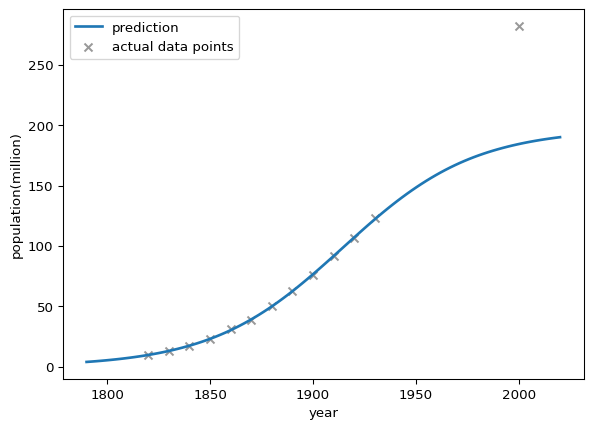
このように, 1800-1930年のアメリカ人口動態を上手く説明するモデルとなっていることがわかります.一方,モデルの上限は \(197\times 10^6\) であるが,2000年の人口は \(282.2\times 10^6\) となっており,長期における人口動態を説明できるものにはなっていないことも読み取れます.
\(N_\infty\) の仮定が間違っていたと解釈することが一つ考えられますが,人口変化を支配する法則は技術変化や政治といった要因に影響を受けるため,常に同じ支配法則に基づいていると仮定することが間違っているとも解釈することが出来ます.