単曲線と追加距離の計算 – regmonkey datascience blog

▶ 基本用語

用語	意味
プラス杭	ナンバー杭間のち底辺株および道路や鉄道の交差部等に設置する点
追加距離	起点からのプラス杭までのトータル距離のこと
接線長	曲線の始点 or 終点から交点(IP)までの距離のこと

基本問題: 曲線の長さを求める

練習 1

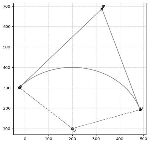
下図に示すような単曲線ABを含む路線の中心線を設置することになった．

扇形 OAB の半径 r = 300
$\displaystyle\angle (IP) = \frac{\pi}{3}$
IP までの追加距離を623(中心杭はAの手前にあるとする)

とする．このとき，曲線の始点 A と曲線の終点 B それぞれの追加距離を求めよ．なお，直線 A(IP) と B(IP) はそれぞれ円の接線であるとする．

コード

import numpy as np
import matplotlib.pyplot as plt


def draw_circle_with_two_tangent(x0, y0, r, ax, theta_start=0, theta_end=2 * np.pi, notations=('O', 'A', 'B', 'IP')):
    # Generate circle points
    theta = np.linspace(theta_start, theta_end, 720)
    x_circle = x0 + r * np.cos(theta)
    y_circle = y0 + r * np.sin(theta)

    # plot
    ax.plot(x_circle, y_circle, "gray", label="Circle (r={radius})")
    ax.plot([x0, x_circle[0]], [y0, y_circle[0]], "gray", linestyle="--")
    ax.plot([x0, x_circle[-1]], [y0, y_circle[-1]], "gray", linestyle="--")
    ax.text(x0, y0, notations[0], verticalalignment="top", horizontalalignment="left")
    ax.scatter(x0, y0, color="k")

    # add text
    ax.text(x_circle[-1], y_circle[-1], notations[1], label="Circle (r={radius})")
    ax.scatter(x_circle[-1], y_circle[-1], color="k")
    ax.text(x_circle[0], y_circle[0], notations[2], label="Circle (r={radius})")
    ax.scatter(x_circle[0], y_circle[0], color="k")

    # plot external intersection points
    mid_theta = (theta_start + theta_end) / 2
    diff_theta = (theta_end - theta_start) / 2 
    external_x = np.cos(mid_theta) * abs(r / np.cos(diff_theta)) + x0
    external_y = np.sin(mid_theta) * abs(r / np.cos(diff_theta)) + y0

    ax.scatter(external_x, external_y, color="k")
    ax.text(external_x, external_y, notations[3], verticalalignment="bottom", horizontalalignment="left")
    ax.plot(
        [external_x, x_circle[0]], [external_y, y_circle[0]], "gray", linestyle="-"
    )
    ax.plot(
        [external_x, x_circle[-1]], [external_y, y_circle[-1]], "gray", linestyle="-"
    )

    return {'A': (x_circle[-1], y_circle[-1]), 'B': (x_circle[0], y_circle[0]), 'IP': (external_x, external_y )}


# params
x0, y0, r0 = 200, 100, 300
theta_start = np.pi / 10
theta_end = np.pi / 10 + np.pi * 2/ 3

fig, ax = plt.subplots(figsize=(6, 6))
coordinates = draw_circle_with_two_tangent(x0, y0, r0, ax, theta_start, theta_end)
ax.grid(True, linestyle="--", alpha=0.6)

Solution

曲線の始点 A の追加距離は

Aの追加距離 = IPの追加距離 − A(IP)の長さ

直線 A(IP) は中心点 O とする円に接しているので

AOの長さ × tan (∠(IP)OA)

接弦定理と円周角の定理より ∠(IP) の外角を I とすると

$$ \begin{align} \angle AOB &= I\\ \angle (IP)OA &= \frac{I}{2} \end{align} $$

したがって，

$$ \text{AOの長さ} \times \tan \frac{I}{2} $$

以上より

$$ \begin{align} A\text{の追加距離} &= 623 - 300 \times \tan \frac{\pi}{3}\\ &= 623 - 300\sqrt{3} \approx 103.4 \end{align} $$

また，Bの追加距離は，弧 AB の長さがわかれば

Bの追加距離 = Aの追加距離 + 弧ABの長さ

と計算できる．

$$ \begin{align} \text{弧}AB\text{の長さ} &= R \times I\\ &= 300 \times \frac{2}{3}\pi\\ &= 200\pi \end{align} $$

したがって，

Bの追加距離 ≈ 103.4 + 628.40 = 731.80

実際にAの追加距離をPythonで近似計算してみると

コード

A, IP = np.array(coordinates['A']), np.array(coordinates['IP'])
A_add_distance = 623 - np.linalg.norm(A - IP)
print(f"Aの追加距離 = {A_add_distance:.2f}")

Aの追加距離 = 103.38

練習 2

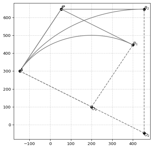
曲線半径 r₁ = 400, $\displaystyle\angle AO_1B = \frac{\pi}{2}$ となるような形で現道路 AB が存在するとする．現在の道路を改良し O₂ を中心とする円曲線からなる新しい道路 AB₂ を建設したいとします．

新しい道路の交点 IP の１は現道路と変わらないとする．

$\displaystyle\angle AO_2B_2 = \frac{\pi}{3}$ としたとき，AB₂ の路線長を求めよ．

コード

# params
x0, y0, r0 = 200, 100, 400
theta_start = np.pi / 3
theta_end = np.pi / 3 + np.pi / 2

fig, ax = plt.subplots(figsize=(6, 6))
coordinates = draw_circle_with_two_tangent(x0, y0, r0, ax, theta_start, theta_end, ('$O_1$', '$A$', '$B_1$', '$IP$'))
ax.grid(True, linestyle="--", alpha=0.6)

r_new = 400 / np.tan(np.pi/6) 
A = np.array(coordinates['A'])
O = np.array((200, 100))
AO = O - A
O_new = A + (AO / np.linalg.norm(AO)) * r_new

coordinates_new = draw_circle_with_two_tangent(*O_new, r_new, ax, theta_end - np.pi/3, theta_end, ('$O_2$', '$A$', '$B_2$', '$IP$'))

Solution

新道路の曲線半径を r₂ としたとき，A(IP) の長さは

$$ \begin{align} A(IP) &= r_1 \times \tan \frac{\pi}{4}\\ &= r_2 \times \tan \frac{\pi}{6} \end{align} $$

と表されるので

$$ \begin{align} r_2 &= \frac{400 \times 1 }{\tan \frac{\pi}{6}}\\ &= 400\times \sqrt{3} &\approx 400\times 1.732\\ &= 692.8 \end{align} $$

したがって，

$$ \text{曲線}AB_2 = 692.8 \times \frac{\pi}{3} \approx 725.1 $$

障害物がある場合の曲線設定

練習 3

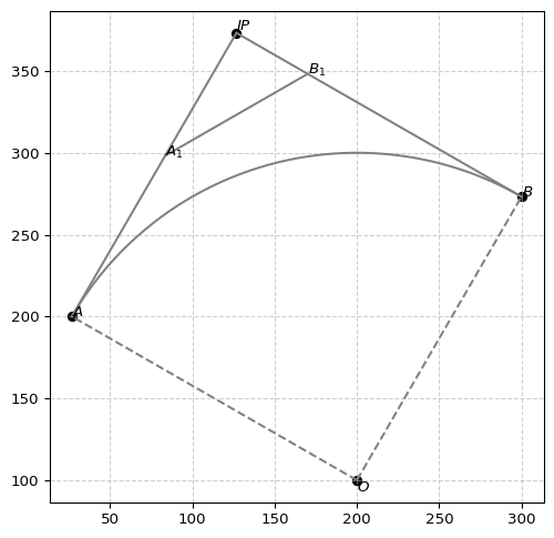
曲線半径 r = 200
A₁B₁ の長さ 100
∠AA₁B₁ = 150^∘
∠BB₁A₁ = 120^∘

という情報が与えられているとき，線分 AA₁ の長さを求めよ．なお，直線 A(IP) と B(IP) はそれぞれ円の接線であるとする．

コード

# params
x0, y0, r0 = 200, 100, 200
theta_start = np.pi / 3
theta_end = theta_start + np.pi / 2

fig, ax = plt.subplots(figsize=(6, 6))
ax.grid(True, linestyle="--", alpha=0.6)

## draw an arc
coordinates = draw_circle_with_two_tangent(x0, y0, r0, ax, theta_start, theta_end, ('$O$', '$A$', '$B$', '$IP$'))

## drar mid-points
B_IP = np.array(coordinates['B']) - np.array(coordinates['IP'])
A_IP = np.array(coordinates['A']) - np.array(coordinates['IP'])
B_1 = np.array(coordinates['IP']) + B_IP / np.linalg.norm(B_IP) * 100 / 2
A_1 = np.array(coordinates['IP']) + A_IP / np.linalg.norm(A_IP) * 100 / 2 * np.sqrt(3)

ax.plot(
        [A_1[0], B_1[0]], [A_1[1], B_1[1]], "gray", linestyle="-"
    )

ax.text(A_1[0], A_1[1], "$A_1$")
ax.text(B_1[0], B_1[1], "$B_1$")

plt.show()

Solution

$\displaystyle\angle AOB = \frac{\pi}{2}$ であるので

length of A(IP) = 200 × tan 45^∘ = 200

正弦定理より

$$ \frac{A_1B_1}{\sin \angle (IP)} = \frac{A_1(IP)}{\sin \angle (IP)B_1A_1} $$

したがって，

$$ \begin{align} \text{length of }A_1(IP) &= 100 \times \sin \angle (IP)B_1A_1\\ &= 100 \times \frac{\sqrt{3}}{2}\\ &\approx 50 \times 1.732 = 86.60 \end{align} $$

以上より

length of AA₁ = 200 − 86.60 = 113.40

Pythonで確認すると

コード

res = np.linalg.norm(np.array(coordinates['A']) - A_1)
print(f"点Aから点A_1までの距離 = {res:.2f}")

点Aから点A_1までの距離 = 113.40