余弦定理の考え方
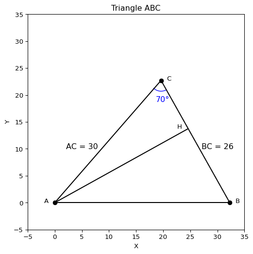
練習 1
\(AC = 30, BC = 26, \angle C = 70^\circ\) となるような \(\triangle ABC\) が与えられたとします.このとき,長さ \(AB\) を求めよ
コード
import matplotlib.pyplot as plt
import numpy as np
import matplotlib.patches as patches

# 辺の長さと角度
AC = 30
BC = 26
angle_C = 70

# 角度をラジアンに変換
angle_C_rad = np.radians(angle_C)

# 点Aの座標
A = (0, 0)

AB = np.sqrt(30**2 + 26**2 - 2 * 30 * 26 * np.cos(np.radians(70)))

# 点Bの座標
B = (AB, 0)

# 点Cの座標
cos_A = (30**2 + AB**2 - 26**2) / (2 * 30 * AB)
sin_A = np.sqrt(1 - cos_A**2)
C = (30 * cos_A, 30 * sin_A)

slope = - (C[0] - B[0])/(C[1] - B[1])
H = (24.6, 24.6 * slope)


# 座標をリストに変換
fig, ax = plt.subplots(figsize=(6, 6))

ax.plot([A[0], H[0]], [A[1], H[1]], "k")  # Black line with circle markers
ax.plot([A[0], B[0]], [A[1], B[1]], "ko-")  # Black line with circle markers
ax.plot([B[0], C[0]], [B[1], C[1]], "ko-")  # Black line with circle markers
ax.plot([C[0], A[0]], [C[1], A[1]], "ko-")  # Black line with circle markers

# 点のラベル
plt.text(H[0]-2, H[1], "H")
plt.text(A[0]-2, A[1], "A")
plt.text(B[0]+1, B[1], "B")
plt.text(C[0]+1, C[1], "C")

# 軸の範囲を設定
plt.xlim(-5, 35)
plt.ylim(-5, 35)

# 軸のラベルを設定
plt.xlabel("X")
plt.ylabel("Y")

# タイトルを設定
plt.title("Triangle ABC")

# Add angles as arcs
arc_radius = 5  # Radius for the arcs

# Angle at B
angle_C_arc = patches.Arc(C, arc_radius*0.8, arc_radius*0.8, angle=250, theta1=np.degrees(320), theta2=np.degrees(70), color='blue')
ax.add_patch(angle_C_arc)
ax.text(C[0]-1, C[1] - arc_radius*.8, f"{70}°", fontsize=12, color='blue')
# ax.text(C[0] + arc_radius/2, B[1] + 1, f"{70}°", fontsize=12, color='blue')
ax.text(5, 10, "AC = 30", fontsize=12, color='black', horizontalalignment='center')
ax.text(30, 10, "BC = 26", fontsize=12, color='black', horizontalalignment='center')

# 図の表示
plt.show()このとき,点 \(A\) から \(BC\) に対して垂線を下ろし,その交点を \(H\) とします.このとき
\[ \begin{align} CH &= AC * \cos(C)\\ BH &= BC - AC * \cos(C)\\ AH& = AC * \sin(C) \end{align} \]
ピタゴラスの定理より
\[ AB^2 = AH^2 + BH^2 \]
なので
\[ \begin{align} AB^2 &= (BC - AC * \cos(C))^2 + (AC * \sin(C))^2\\ &= BC^2 + AC^2 - 2\cdot BC\cdot AC \cos(C) \end{align} \]
従って,
コード
print(f"AB = {AB:.2f}")AB = 32.29▶ ベクトルを用いた直感的理解
ベクトルの内積は \(\vec a \cdot \vec b = \lvert a \rvert \lvert b \rvert \cos \theta\) で定義されることを利用すると,
\[ \begin{aligned} AB^2 &= \left\lvert \overrightarrow{CA} - \overrightarrow{CB} \right\rvert^2 \\ &= (\overrightarrow{CA} - \overrightarrow{CB}) \cdot (\overrightarrow{CA} - \overrightarrow{CB}) \\ &= \left\lvert \overrightarrow{CA} \right\rvert^2 + \left\lvert \overrightarrow{CB} \right\rvert^2 - 2 \overrightarrow{CA} \cdot \overrightarrow{CB} \\ &= \left\lvert \overrightarrow{CA} \right\rvert^2 + \left\lvert \overrightarrow{CB} \right\rvert^2 - 2 \left\lvert \overrightarrow{CA} \right\rvert \left\lvert \overrightarrow{CB} \right\rvert \cos(\angle ACB) \\ &= AC^2 + BC^2 - 2\cdot AC\cdot BC \cos(C) \end{aligned} \]
正弦定理と余弦定理の応用: 対岸の2点間距離を測る
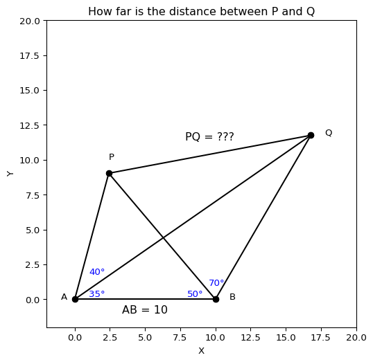
練習 2
四角形PABQ が以下のように与えられている
- \(AB = 10\)
- \(\angle PAB = {75}^\circ\)
- \(\angle PBA = {50}^\circ\)
- \(\angle PAQ = {40}^\circ\)
- \(\angle QAB = {35}^\circ\)
- \(\angle PBQ = {70}^\circ\)
このとき,PQの距離を求めよ.
コード
import matplotlib.pyplot as plt
import numpy as np
import matplotlib.patches as patches

# 辺の長さと角度
AB = 10
angle_PAB = np.radians(75)
angle_PBA = np.radians(50)
angle_QAB = np.radians(35)
angle_AQB = np.radians(25)
angle_QBA = np.radians(120)
angle_APB = np.radians(55)


# 点Aの座標
A = (0, 0)

# 点Bの座標
B = (AB, 0)

# 点Pの座標
PA = AB / np.sin(angle_APB) * np.sin(angle_PBA)
P = ((np.cos(angle_PAB)) * PA, (np.sin(angle_PAB)) * PA)

# 点Qの座標
QA = AB / np.sin(angle_AQB) * np.sin(angle_QBA)
Q = ((np.cos(angle_QAB)) * QA, (np.sin(angle_QAB)) * QA)


# 座標をリストに変換
fig, ax = plt.subplots(figsize=(6, 6))

ax.plot([A[0], P[0]], [A[1], P[1]], "k")  # Black line with circle markers
ax.plot([A[0], B[0]], [A[1], B[1]], "ko-")  # Black line with circle markers
ax.plot([B[0], P[0]], [B[1], P[1]], "ko-")  # Black line with circle markers
ax.plot([Q[0], A[0]], [Q[1], A[1]], "ko-")  # Black line with circle markers
ax.plot([Q[0], B[0]], [Q[1], B[1]], "ko-")  # Black line with circle markers
ax.plot([Q[0], P[0]], [Q[1], P[1]], "ko-")  # Black line with circle markers

# 点のラベル
plt.text(A[0] - 1, A[1], "A")
plt.text(B[0] + 1, B[1], "B")
plt.text(P[0], P[1] + 1, "P")
plt.text(Q[0] + 1, Q[1], "Q")

# 軸の範囲を設定
plt.xlim(-2, 20)
plt.ylim(-2, 20)

# 軸のラベルを設定
plt.xlabel("X")
plt.ylabel("Y")

# タイトルを設定
plt.title("How far is the distance between P and Q")

# Add angles as arcs
arc_radius = 5  # Radius for the arcs

# Angle at B
ax.text(A[0] + 1, A[1] + 1.8, f"{40}°", fontsize=10, color="blue")
ax.text(A[0] + 1, A[1] + 0.2, f"{35}°", fontsize=10, color="blue")
ax.text(B[0] - 2, B[1] + 0.2, f"{50}°", fontsize=10, color="blue")
ax.text(B[0] - 0.5, B[1] + 1, f"{70}°", fontsize=10, color="blue")
# ax.text(C[0] + arc_radius/2, B[1] + 1, f"{70}°", fontsize=12, color='blue')
ax.text(5, -1, "AB = 10", fontsize=12, color="black", horizontalalignment="center")
ax.text(
    (P[0] + Q[0]) / 2,
    (P[1] + Q[1]) / 2 + 1,
    "PQ = ???",
    fontsize=12,
    color="black",
    horizontalalignment="center",
)


# 図の表示
plt.show()