カバリエリの原理

カバリエリの原理

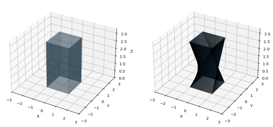
一辺長さ \(2\) の正方形を底面として高さ3の直方体と，それをちょっとずつねじる形でずらした立体を以下のように考えます． 右図において，\(xy\) 平面に並行な各断面はどれも等しく一辺の長さ \(2\) の正方形で，その面積は \(4\) となってるとします．

このとき，カバリエリの原理よりどちらの立体像の体積は等しいことが言えます．

import numpy as np
import matplotlib.pyplot as plt
from mpl_toolkits.mplot3d.art3d import Poly3DCollection


def plot_cuboid(data, length=2, width=2, height=3, ax=None):
    if ax is None:
        fig = plt.figure()
        ax = fig.add_subplot(111, projection="3d")
    poly3d = Poly3DCollection(data, alpha=0.2, edgecolor="k")
    ax.add_collection3d(poly3d)

    # Set limits
    max_dim = max(length, width, height)
    ax.set_xlim([-max_dim, max_dim])
    ax.set_ylim([-max_dim, max_dim])
    ax.set_zlim([0, height * 1.1])
    ax.set_xlabel("X")
    ax.set_ylabel("Y")
    ax.set_zlabel("Z")


def twisted_cuboid(
    length=2, width=2, height=3, twist_angle=np.pi / 2, num_segments=500
):
    # Define the base (bottom) of the cuboid
    base_vertices = np.array(
        [
            [-length / 2, -width / 2, 0],
            [length / 2, -width / 2, 0],
            [length / 2, width / 2, 0],
            [-length / 2, width / 2, 0],
        ]
    )

    # Define the top face with a twist
    rotation_matrix = np.array(
        [
            [np.cos(twist_angle), -np.sin(twist_angle), 0],
            [np.sin(twist_angle), np.cos(twist_angle), 0],
            [0, 0, 1],
        ]
    )
    top_vertices = base_vertices @ rotation_matrix.T + np.array([0, 0, height])

    # Interpolate between base and top vertices
    vertices = []
    for i in range(num_segments + 1):
        t = i / num_segments
        interpolated_vertices = (1 - t) * base_vertices + t * top_vertices
        vertices.append(interpolated_vertices)
    vertices = np.vstack(vertices)

    # Define faces
    faces = []
    for i in range(num_segments):
        for j in range(4):
            next_j = (j + 1) % 4
            faces.append(
                [
                    vertices[i * 4 + j],
                    vertices[i * 4 + next_j],
                    vertices[(i + 1) * 4 + next_j],
                    vertices[(i + 1) * 4 + j],
                ]
            )

    return faces


def cuboid(length=2, width=2, height=3, num_segments=100, ax=None):
    # Define the base (bottom) of the cuboid
    base_vertices = np.array(
        [
            [-length / 2, -width / 2, 0],
            [length / 2, -width / 2, 0],
            [length / 2, width / 2, 0],
            [-length / 2, width / 2, 0],
        ]
    )

    # Define the top face without a twist
    top_vertices = base_vertices + np.array([0, 0, height])

    # Interpolate between base and top vertices
    vertices = []
    for i in range(num_segments + 1):
        t = i / num_segments
        interpolated_vertices = (1 - t) * base_vertices + t * top_vertices
        vertices.append(interpolated_vertices)
    vertices = np.vstack(vertices)

    # Define faces
    faces = []
    for i in range(num_segments):
        for j in range(4):
            next_j = (j + 1) % 4
            faces.append(
                [
                    vertices[i * 4 + j],
                    vertices[i * 4 + next_j],
                    vertices[(i + 1) * 4 + next_j],
                    vertices[(i + 1) * 4 + j],
                ]
            )

    return faces


# compute points
cuboid_records = cuboid()
twisted_cuboid_records = twisted_cuboid()

# plots
fig = plt.figure(figsize=(12, 6))
ax1 = fig.add_subplot(121, projection="3d")
ax2 = fig.add_subplot(122, projection="3d")

plot_cuboid(cuboid_records, ax=ax1)
plot_cuboid(twisted_cuboid_records, ax=ax2)

plt.show()

Theorem 1 : カバリエリの原理

2つの立体について，平行な平面で切った切り口を比べる．互いの面積がいつも等しいならば，この２つの立体の体積は等しい．

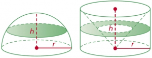
半径 \(r\) の円を底面とする高さ \(h\) の円柱を考えます． なお \(h = r\) とします．この円柱から，半径 \(r\) の円を底面とする円錐を以下のように抜き取った立体を作ります（以降，穴あき円柱と呼ぶ）．

カバリエリの原理

この穴開き円柱の体積は

\[ \begin{align} \pi r^2\times h - \pi r^2\times \frac{h}{3} &= \frac{2}{3} \pi r^2 h \end{align} \]

一方，半径 \(r\) の半球の体積は

\[ \begin{align} \frac{1}{2} \times \frac{4}{3}\pi r^3 = \frac{2}{3} \pi r^2h \end{align} \]

２つの立体の体積が一致することがわかります．これをカバリエリの原理を使って確かめてみます．

まず穴あき円錐について，高さ \(a \in [0, h]\) における断面積（緑色の部分）は

\[ r^2\pi - \left(\frac{a}{r}r\right)^2\pi = (r^2 - a^2)\pi \]

半球の方は，ピタゴラスの定理より高さ \(a\) のときの半径が \(\sqrt{r^2 - a^2}\) と求まるので

\[ (\sqrt{r^2 - a^2})^2\pi = (r^2 - a^2)\pi \]

従って，２つの立体について任意の高さ \(a \in [0, h]\) において互いの面積がいつも等しいことがわかります．

ずらし変形で面積を求める

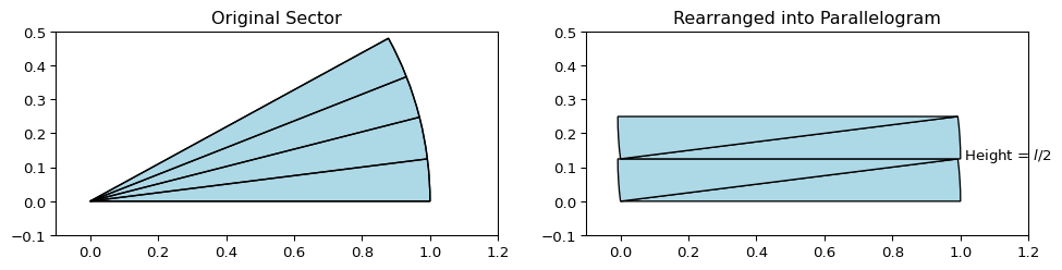
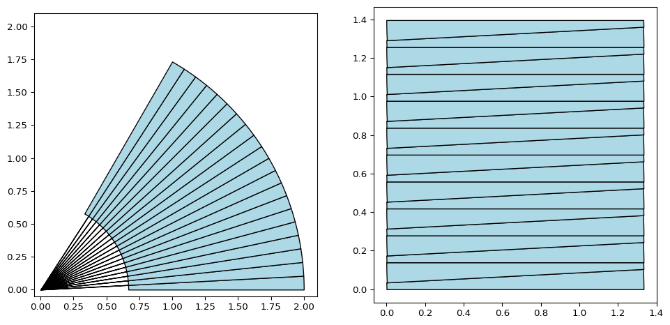
半径 \(r\), 弧の長さ \(l\) の扇形の面積を求めたいとします．扇形に対し，分割交互ずらしをして以下のように長方形へ極限等積変形を実施します．

import numpy as np
import matplotlib.pyplot as plt
from matplotlib.patches import Wedge, Polygon

# Parameters
r = 1  # radius
l = 0.5  # arc length

# Calculate the angle of the sector
theta = l / r  # in radians
divide_num = 4

# Create the sector
fig, ax = plt.subplots(1, 2, figsize=(12, 6))

# Plot the original sector
sector = Wedge(
    (0, 0), r, 0, np.degrees(theta), facecolor="lightblue", edgecolor="black"
)
ax[0].add_patch(sector)
ax[0].set_xlim(-0.1, r * 1.2)
ax[0].set_ylim(-0.1, l)
ax[0].set_aspect("equal", "box")
ax[0].set_title("Original Sector")

# Divide the sector into four parts
angles = np.linspace(0, theta, divide_num+1)
for i in range(divide_num):
    wedge = Wedge(
        (0, 0),
        r,
        np.degrees(angles[i]),
        np.degrees(angles[i + 1]),
        facecolor="none",
        edgecolor="black",
    )
    ax[0].add_patch(wedge)

# Rearrange the parts into a parallelogram

# Create the parallelogram by shifting the parts
for i in range(divide_num):
    if i % 2 == 0:
        sector = Wedge(
            (0, np.sin(theta / divide_num) * (i // 2)), r, 0, np.degrees(theta / divide_num), facecolor="lightblue", edgecolor="black"
        )
    else:
        sector = Wedge(
            (np.cos(theta / divide_num), np.sin(theta / divide_num) * (i // 2 + 1 )),
            r,
            np.degrees(np.pi),
            np.degrees(theta / divide_num + np.pi),
            facecolor="lightblue",
            edgecolor="black",
        )
    ax[1].add_patch(sector)
    

# add info
ax[1].text(1.01, l/4, f"Height = $l/2$", horizontalalignment="left")

ax[1].set_xlim(-0.1, r * 1.2)
ax[1].set_ylim(-0.1, l)
ax[1].set_aspect("equal", "box")
ax[1].set_title("Rearranged into Parallelogram")

plt.show()

上の図では４分割ですが，これを細かくすると横の長さ \(r\), 縦の長さ \(l/2\) の長方形へ変形することができるとみなせるので

\[ S = \frac{l}{2}r \]

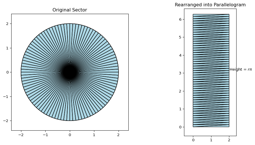
と計算することが出来ます．半径 \(r\), 弧の長さ \(l = 2\pi r\) のとき，扇形は円になりますが，その円の面積も同様に

\[ S = \frac{2\pi r}{2}r = r^2 \pi \]

と計算でき，円の面積の公式と一致することがわかります

import numpy as np
import matplotlib.pyplot as plt
from matplotlib.patches import Wedge, Polygon

# Parameters
r = 2  # radius
l = 2*np.pi * r  # arc length

# Calculate the angle of the sector
theta = l / r  # in radians
divide_num = 100

# Create the sector
fig, ax = plt.subplots(1, 2, figsize=(12, 6))

# Plot the original sector
sector = Wedge(
    (0, 0), r, 0, np.degrees(theta), facecolor="lightblue", edgecolor="black"
)
ax[0].add_patch(sector)
ax[0].set_xlim(-r * 1.2, r * 1.2)
ax[0].set_ylim(-r * 1.2, r * 1.2)
ax[0].set_aspect("equal", "box")
ax[0].set_title("Original Sector")

# Divide the sector into four parts
angles = np.linspace(0, theta, divide_num+1)
for i in range(divide_num):
    wedge = Wedge(
        (0, 0),
        r,
        np.degrees(angles[i]),
        np.degrees(angles[i + 1]),
        facecolor="none",
        edgecolor="black",
    )
    ax[0].add_patch(wedge)

# Rearrange the parts into a parallelogram

# Create the parallelogram by shifting the parts
for i in range(divide_num):
    if i % 2 == 0:
        sector = Wedge(
            (0, np.sin(theta / divide_num) * (i // 2)* r), r, 0, np.degrees(theta / divide_num), facecolor="lightblue", edgecolor="black"
        )
    else:
        sector = Wedge(
            (np.cos(theta / divide_num)* r, np.sin(theta / divide_num) * r * (i // 2 + 1 )),
            r,
            np.degrees(np.pi),
            np.degrees(theta / divide_num + np.pi),
            facecolor="lightblue",
            edgecolor="black",
        )
    ax[1].add_patch(sector)
    

# add info
ax[1].text(r + 0.01, l/4, f"Height = $r\pi$", horizontalalignment="left")

ax[1].set_xlim(-0.5, r * 1.2)
ax[1].set_ylim(-0.5, l/2 * 1.05)
ax[1].set_aspect("equal", "box")
ax[1].set_title("Rearranged into Parallelogram")

plt.show()

パイン形とずらし面積

半径 \(2\), 弧の長さが \(\displaystyle L = \frac{2}{3}\pi\) の扇形から，半径 \(2/3\), 弧の長さが \(\displaystyle l = \frac{2}{9}\pi\) の扇形を除いたパイン形を考えます．このパイン形に対して，「分割交互ずらし」を適用して極限を取ると，底辺の長さ \(\displaystyle \frac{4}{3}\)，高さ

\[ \text{height} = \frac{l + L}{2} = \frac{4}{9}\pi \]

の長方形へ収束します．このとき，このパイン型の面積は

\[ S = \frac{l + L}{2}\times \frac{4}{3} = \frac{16}{27}\pi \]

import numpy as np
import matplotlib.pyplot as plt
from shapely.geometry import Polygon
from shapely.affinity import translate
from shapely.ops import unary_union
from shapely.affinity import rotate
import geopandas as gpd


def create_sector(center, radius, angle_start, angle_end, num_points=100):
    """Creates a sector shape as a polygon using Shapely."""
    angles = np.linspace(np.radians(angle_start), np.radians(angle_end), num_points)
    outer_arc = [
        (center[0] + radius * np.cos(a), center[1] + radius * np.sin(a)) for a in angles
    ]
    return Polygon([center] + outer_arc + [center])  # Close the polygon


# Parameters
divide_num = 20
ring_sector_list = []
outer_radius = 2
angle = 60 / divide_num

for i in range(divide_num):
    center = (0, 0)
    inner_radius = outer_radius / 3
    angle_start, angle_end = angle * i, angle * (i + 1)  # Angle in degrees

    # Create outer and inner sectors
    outer_sector = create_sector(center, outer_radius, angle_start, angle_end)
    inner_sector = create_sector(center, inner_radius, angle_start, angle_end)

    # Subtract inner sector from outer sector to get the ring shape
    ring_sector = outer_sector.difference(inner_sector)
    ring_sector_list.append(ring_sector)


# plot
fig, ax = plt.subplots(1, 2, figsize=(12, 6))

for ring_sector in ring_sector_list:
    # Plot using GeoPandas
    gdf = gpd.GeoSeries([ring_sector])
    gdf.plot(ax=ax[0], color="lightblue", edgecolor="black")

# Formatting
ax[0].set_xlim(-0.05, outer_radius + 0.1)
ax[0].set_ylim(-0.05, outer_radius + 0.1)

gdf = gpd.GeoSeries([ring_sector_list[0]])
rotated_gdf = gpd.GeoSeries(rotate(ring_sector_list[0], 180, origin="center"))
for i in range(len(ring_sector_list)):
    # Plot using GeoPandas
    if i % 2 == 0:
        gdf_tmp = gdf.apply(
            lambda geom: translate(
                geom, xoff=-2/3, yoff=np.sin(np.radians(angle))*8/3 * (i//2)
            )
        )
        gdf_tmp.plot(ax=ax[1], color="lightblue", edgecolor="black")
    else:
        gdf_tmp = rotated_gdf.apply(
            lambda geom: translate(
                geom, xoff=-2/3, yoff=np.sin(np.radians(angle))*2/3 * (i//2 + 1) + np.sin(np.radians(angle))*6/3 * (i//2)
            ))
        gdf_tmp.plot(ax=ax[1], color="lightblue", edgecolor="black")


plt.show()

線分の運動とずらし面積

野球グラウンドをならすときトンボという道具を使ったりします．このトンボを引きづる用な形でグラウンドを適当に歩くと，トンボがなす線分がグラウンドを通過することで図形が出来ます． 線分の運動の観点から，この図形の面積を求める方法をここでは紹介します．

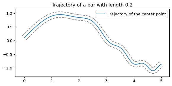
from scipy import interpolate
import numpy as np
import matplotlib.pyplot as plt

N = 1000

x = np.linspace(0, 5, N)

y = (
    np.sin(x)
    + np.cos(x ** 2) / 10
)

dydx = np.cos(x) - (2 / 10) * np.sin(x ** 2) * x
dydx = np.where(abs(dydx) > 1e-10, dydx, 0)


upper_x = []
upper_y = []
lower_x = []
lower_y = []

for i in range(N):
    if dydx[i] < 0:
        dy = abs(1/dydx[i])
        dist = np.sqrt(dy**2 + 1) * 10
        dx = 1 / dist
        dy = dy / dist
    elif dydx[i] > 0:
        dy = abs(1/dydx[i])
        dist = np.sqrt(dy**2 + 1)  * 10
        dx = -1/ dist
        dy = dy / dist
    else:
        dx, dy = (0, 1 / 10)
    
    upper_y.append(y[i] + dy)
    upper_x.append(x[i] + dx)
    lower_y.append(y[i] - dy)
    lower_x.append(x[i] - dx)

fig, ax = plt.subplots()

ax.plot(x, y, label = 'Trajectory of the center point')
ax.plot(upper_x, upper_y, color='gray', linestyle='--')
ax.plot(lower_x, lower_y, color='gray', linestyle='--')

ax.set_aspect('equal', 'box')  # Ensure the x and y axes have the same ratio

ax.set_title("Trajectory of a bar with length 0.2")

plt.legend()
plt.show()

一般に，大きさのある物体（剛体という）の運動は，「並進運動」と「回転運動」の合成で表されます．長さ \(0.2\) のトンボがグラウンドを並進運動と回転運動で通過する際に描かれる図形をplotしたものが上の図となります． 灰色の点線がそれぞれトンボの両端の軌跡を描いており，青の実線がトンボの中心点の軌跡となります．トンボがならしたグラウンドの面積は灰色で囲まれたエリアとなります．

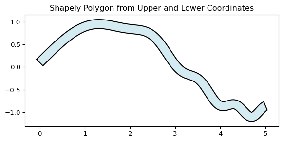
▶  shapely.Polygonを用いた面積の計算

上記で中心点の軌跡から両端の軌跡の座標を計算してあるので，それらを用いて shapely.Polygon をまず定義します．

# shapely.Polygonの設定
polygon_coords = list(zip(upper_x, upper_y)) + list(zip(lower_x[::-1], lower_y[::-1]))
polygon = Polygon(polygon_coords)

# Plot the polygon
fig, ax = plt.subplots()
x, y = polygon.exterior.xy
ax.plot(x, y, color='black')
ax.fill(x, y, color='lightblue', alpha=0.5)
ax.set_title("Shapely Polygon from Upper and Lower Coordinates")
ax.set_aspect('equal', 'box')  # Ensure the x and y axes have the same ratio
plt.show()

その後，Polygon によって定義された図形の面積を計算すれば良いので

polygon.area

1.2470071445781767

▶  曲線の長さの公式と線分の移動

詳しい説明はのちの機会としますが，線分が履く面積は

\[ \text{線分がはく面積} = \text{中点の移動距離} \times \text{線分の長さ} \]

で計算することが出来ます．線分の長さは \(0.2\) とわかっているので，「中点の移動距離」を求めれば面積が求まりそうなことがわかります．

Theorem 2 : 曲線の長さ

\(y=f(x)\) で表される曲線の \(x \in [a, b]\) の部分の長さ \(L\) は，

\[ L = \int^b_a \sqrt{1 + f^\prime(x)^2} dx \]

​（ただし，\(f(x)\) は微分可能で \(f^\prime(x)\) は連続とする）

点 \(x\) から\(\Delta x\) 動いたとき，\(\Delta y \approx f^\prime(x)\Delta x\) 動くことから，その区間での曲線の長さは

\[ \sqrt{(\Delta x)^2 + (f^\prime(x)\Delta x)^2} = \sqrt{1 + f^\prime(x)^2}\Delta x \]

で近似できます．従って，\(\Delta x \to dx\) と極限を取ることで

\[ L = \int^b_a \sqrt{1 + f^\prime(x)^2} dx \]

と理解することが出来ます．

今回の曲線 \(f(x)\) は \([0, 5]\) 区間で以下のように記述することができるとします．

\[ f(x) = \sin(x) + 0.1\cos(x^2) \]

このとき，\(f(x)\) の1次導関数は

\[ f^\prime(x) = \cos(x) - 0.2 x \sin(x^2) \]

従って，曲線の公式より

\[ L = \int^5_0 \sqrt{1 + \cos^2(x) + 0.04 x^2 \sin^2(x^2) - 0.4x\cos(x)\sin(x^2)}dx \]

scipy.integrate.quad を用いて数値計算すると

from scipy.integrate import quad


def curve_length(x):
    return np.sqrt(
        np.cos(x) ** 2
        + 1 / 25 * np.sin(x**2) ** 2 * x**2
        - 2 / 5 * np.cos(x) * np.sin(x**2) * x
        + 1
    )


print(quad(curve_length, 0, 5)[0] * 0.2)

1.24703476690297

shapely.Polygon を用いた計算結果と近しい値であることから計算結果の妥当性をうかがい知ることができます．