円の式
\((a, b)\) を中心点とする半径 \(r\) の円をplotすることを考えます.
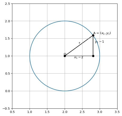
半径 \(r\) の円の中心点の座標が原点 \((0, 0)\) にある場合,円周上の点 \(P = (x, y)\) は,\(P\) から \(x\) 軸に下ろした垂線と \(x\) 軸が交わる点を \(Q\) としたとき \(\triangle OPQ\) は斜辺 \(r\) ,高さ \(y\) , 底辺の長さ \(x\) となる直角三角形を構成するので,三平方の定理より
\[
r^2 = x^2 + y^2
\]
これが円上の座標が満たす方程式となります.原点を中心点とする場合を考えましたが,中心が \((a, b)\) ,半径 \(r\) の円の式は同様の方法で
\[
r^2 = (x - a)^2 + (y - b)^2 \label{#eq-circle}
\]
と表すことが出来ます.
コード
import matplotlib.pyplot as pltimport numpy as npimport matplotlib.tri as mtri# set params = 1 = (2 , 1 )# variables = np.linspace(0 , 2 * np.pi, 1000 )= np.cos(theta) * R + O[0 ]= np.sin(theta) * R + O[1 ]= (x[100 ], y[100 ])= [[0 , 1 , 2 ]]= [O[0 ], A[0 ], A[0 ]]= [O[1 ], O[1 ], A[1 ]]= mtri.Triangulation(x_trinagle, y_trinagle, triangles)# plot = plt.subplots(figsize= (8 , 6 ))"equal" )0.5 , 3.5 )- 0.5 , 2.5 )* O, s= 8 , color= "k" )* A, s= 8 , color= "k" )* O, s= "O" , ha= 'center' , va= 'bottom' )* A, s= "A = ($x_1, y_1$)" , ha= 'left' , va= 'bottom' )2.4 , 1.35 , s= "r" )2.4 , 0.9 , s= "$x_1 - 2$" , ha= 'center' , va= 'bottom' )0 ]+ 0.05 , 1.35 , s= "$y_1 - 1$" , ha= 'left' , va= 'bottom' )# add lines 'ko-' )
3点を通る円の方程式
コード
# set params = 2.5 = (3 , 1 / 2 )# variables = np.linspace(0 , 2 * np.pi, 1000 )= np.cos(theta) * R + O[0 ]= np.sin(theta) * R + O[1 ]= (1 , - 1 )= (3 , 3 )= (1 , 2 )# plot = plt.subplots(figsize= (8 , 6 ))"equal" )* O, s= 8 , color= "k" )* P, s= 8 , color= "k" )* Q, s= 8 , color= "k" )* R, s= 8 , color= "k" )* O, s= "O" , ha= 'center' , va= 'bottom' )* P, s= "P" , ha= 'center' , va= 'bottom' )* Q, s= "Q" , ha= 'left' , va= 'bottom' )* R, s= "R" , ha= 'left' , va= 'bottom' )
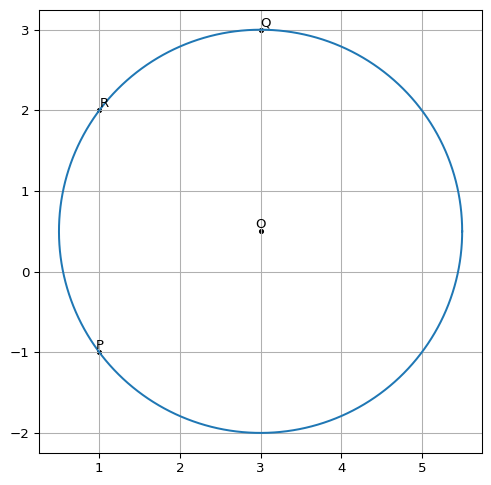
3点 \(P = (1, -1), Q = (3, 3), R = (1, 2)\) が与えられたとして,この3点を通る円を求める問題を考えます.
\(\eqref{#eq-circle}\) を展開すると
\[
x^2 + y^2 - 2ax - 2by + a^2 + b^2 = r^2
\]
これを整理して
\[
x^2 + y^2 + Ax + By + C = 0 \label{#eq-basemodel}
\]
と変形します.ここで,\(P = (1, -1), Q = (3, 3), R = (1, 2)\) の情報を用いると
\[
\begin{gather}
2 + A - B + C = 0\\
18 + 3A + 3B + C = 0\\
5 + A +2B + C = 0
\end{gather}
\]
という \(A,B,C\) についての連立方程式を得ることが出来ます.これを解くと
\[
A = -6, B = -1, C = 3
\]
従って,
\[
(x - 3)^2 + (y - 0.5)^2 = 2.5^2 \label{#eq-ans1}
\]
外接円から求める
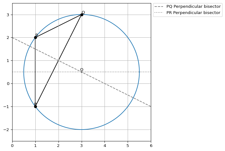
点 \(P, Q, R\) からなる三角形の外接円として求めたい円を捉えることも出来ます. 外接円の円心は三角形の各線分の垂直二等分線の交点として求めることが出来ます.
コード
def func_pq(x):= - (P[0 ] - Q[0 ]) / (P[1 ] - Q[1 ])= - a * (P[0 ] + Q[0 ]) / 2 + (P[1 ] + Q[1 ]) / 2 return a* x + bdef func_pr(x):= - (P[0 ] - R[0 ]) / (P[1 ] - R[1 ])= - a * (P[0 ] + R[0 ]) / 2 + (P[1 ] + R[1 ]) / 2 return a* x + b= np.array([0 , 6 ])= [[0 , 1 , 2 ]]= [P[0 ], Q[0 ], R[0 ]]= [P[1 ], Q[1 ], R[1 ]]= mtri.Triangulation(x_trinagle, y_trinagle, triangles)# plot = plt.subplots(figsize= (8 , 6 ))"equal" )0 , 6 )- 2.5 , 3.5 )= 'PQ Perpendicular bisector' , linestyle= '--' , color= 'gray' )= 'PR Perpendicular bisector' , linestyle= ':' , color= 'gray' )* O, s= 8 , color= "k" )* P, s= 8 , color= "k" )* Q, s= 8 , color= "k" )* R, s= 8 , color= "k" )* O, s= "O" , ha= 'center' , va= 'bottom' )* P, s= "P" , ha= 'center' , va= 'bottom' )* Q, s= "Q" , ha= 'left' , va= 'bottom' )* R, s= "R" , ha= 'left' , va= 'bottom' )# add lines 'ko-' )= 'center left' , bbox_to_anchor= (1 , 0.95 ))
\(PQ\) の垂直二等分線 \(f(x)\) は
\[
\begin{align}
f(x)
&= -\frac{P_x - Q_x}{P_y - Q_y}x + \frac{P_y + Q_y}{2} + \frac{P_x - Q_x}{P_y - Q_y} \frac{P_x + Q_y}{2}\\
&= -\frac{P_x - Q_x}{P_y - Q_y}x + \frac{P_x^2 - Q_x^2 + P_y^2 - Q_y^2}{2(P_y - Q_y)}
\end{align}
\]
同様に \(PR\) の垂直二等分線 \(g(x)\) は
\[
\begin{align}
g(x)
&= -\frac{P_x - R_x}{P_y - R_y}x + \frac{P_y + R_y}{2} + \frac{P_x - R_x}{P_y - R_y} \frac{P_x + R_y}{2}\\
&= -\frac{P_x - R_x}{P_y - R_y}x + \frac{P_x^2 - R_x^2 + P_y^2 - R_y^2}{2(P_y - R_y)}
\end{align}
\]
ここから \(f(x), g(x)\) が交差する点を求めることで外接円の円心を求めることが出来ます.
少しめんどくさいので,数値計算で説いてみると
コード
= - (P[0 ] - Q[0 ]) / (P[1 ] - Q[1 ])= - a * (P[0 ] + Q[0 ]) / 2 + (P[1 ] + Q[1 ]) / 2 = - (P[0 ] - R[0 ]) / (P[1 ] - R[1 ])= - c * (P[0 ] + R[0 ]) / 2 + (P[1 ] + R[1 ]) / 2 print ((d- b)/ (a- c), a * (d- b)/ (a- c) + b)
\(\eqref{#eq-ans1}\) と一致する計算結果となることが確かめられました.
📘 REMARKS
上記の垂直二等分線の交点を \((x_0, y_0)\) としたとき,整理すると以下のようになります.
\[
A = \left(\begin{array}{cc}
R_y - Q_y & -(P_y - Q_y)\\
-(R_x - Q_x) & P_x - Q_x\\
\end{array}\right)
\]
としたとき,
\[
\left(\begin{array}{c}
x_0\\
y_0
\end{array}\right)
= \frac{1}{\operatorname{det}A} A\left(\begin{array}{c}
(P_x^2 - Q_x^2 + P_y^2 - Q_y^2)/2\\
(R_x^2 - Q_x^2 + R_y^2 - Q_y^2)/2
\end{array}\right)
\]
実際に計算してみると
コード
= np.array([[R[1 ] - Q[1 ], - (P[1 ] - Q[1 ])], [- (R[0 ] - Q[0 ]), P[0 ] - Q[0 ]]])= np.array(0 ]** 2 - Q[0 ]** 2 + P[1 ]** 2 - Q[1 ]** 2 ) / 2 ],0 ]** 2 - Q[0 ]** 2 + R[1 ]** 2 - Q[1 ]** 2 ) / 2 ],= np.ravel((A_array @ B_array) / np.linalg.det(A_array))= np.sqrt(np.sum ((np.array(P) - result) ** 2 ))print (f"中心点 = ( { result} ), 半径 = { radius} " )
中心点 = ([3. 0.5]), 半径 = 2.5
敵の砲台の座標を探せ
練習 1
とある固定の1地点から自軍領地に対して敵が砲撃をかけてきているとします. 敵の砲台は角度のみを調整できるだけで,砲撃予定距離 \(r\) は一定とします.ただし,実際の砲撃距離は風向などの外乱要因によってノイズが混じっているとします.
とある日に敵から50回の攻撃を受けたとき,その砲台座標を推定してください.砲撃のノイズは\(\operatorname{i.i.d}\) とする.
\(\eqref{#eq-basemodel}\) より
\[
\begin{align}
z_i = - x_i^2 - y_i^2
\end{align}
\]
と定義すると,\(e_i\) をresidualとして
\[
z_i = \beta_0 + \beta_1 x_i + \beta_2 y_i + e_i
\]
について \((\beta_0, \beta_1, \beta_2)\) をLinear modelで推定し,その推定値を \((\hat\beta_0, \hat\beta_1, \hat\beta_2)\) と表せば 敵の砲台の推定座標 \((\hat x, \hat y)\) 及び推定距離 \(\hat r\) は
\[
\begin{align}
\hat x &= -\hat\beta_1/2\\
\hat y &= -\hat\beta_2/2\\
\hat r &= \sqrt{\hat x^2 + \hat y^2 - \hat\beta_0}
\end{align}
\]
と計算できそうに思えます.
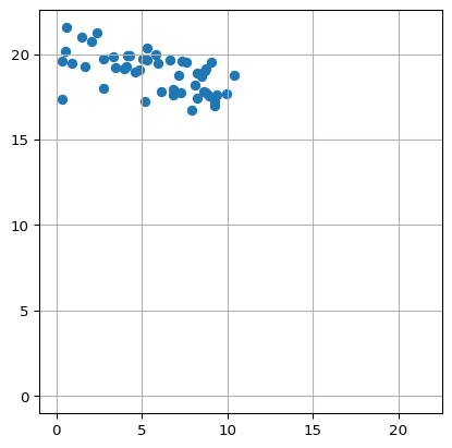
▶ Data Generating Process
敵の砲台の座標は \((0, 0)\)
敵は \((0, 0)\) の地点から砲撃距離 \(20\) で攻撃してくる
実際の砲撃距離 \(r \sim N(20, 1)\)
砲撃角度は \(\left[\displaystyle{\frac{\pi}{3}, \frac{\pi}{2}}\right]\) の範囲で一様分布で定まる
というData Generating Processとします.
コード
def gdp(x_0: float , y_0: float , noise: float = 1.0 , radius: float = 20 , attack_num: int = 50 ):# params = np.random.uniform(np.pi/ 3 , np.pi/ 2 , attack_num)= radius + np.random.normal(0 , noise, attack_num)= np.cos(theta) * r + x_0= np.sin(theta) * r + y_0return x, y
このGDPに従う形で攻撃されたとするとき,その散布図は以下のようになります.
コード
42 )= gdp(0 , 0 )= plt.subplots()- 1 , np.max ([np.max (x_attack), np.max (y_attack)]) + 1 )- 1 , np.max ([np.max (x_attack), np.max (y_attack)]) + 1 )'equal' )
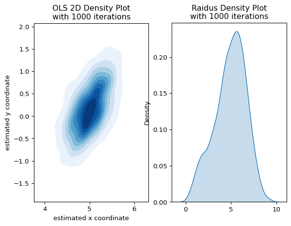
▶ OLS Monte Carlo Simulation
OLSによるパラメータ推定値を \(1,000\) 回simulationし,その組み合わせをkde plotしたものが以下となります.x座標についてバイアスがあることがわかります. 砲撃距離に関しても不自然な推定値となっています.
コード
import pandas as pdimport statsmodels.api as smimport seaborn as snsdef gpd_dataframe(x: float = 0 , y: float = 0 , noise: float = 1.0 ):= gdp(x, y, noise)= pd.DataFrame("x_coordinate" : x_attack,"y_coordinate" : y_attack,return dfdef ols_solver(tuple [str ] = ("x_coordinate" , "y_coordinate" )= - (df[xy_columns[0 ]] ** 2 ) - df[xy_columns[1 ]]= sm.add_constant(df.loc[:, xy_columns])# regression = sm.OLS(Y, X)= model.fit()# convert estimates to target params = - results.params[xy_columns[0 ]] / 2 = - results.params[xy_columns[1 ]] / 2 = (x_hat** 2 + y_hat** 2 - results.params['const' ])= np.sqrt(r_hat_sqr) if r_hat_sqr > 0 else np.nanreturn [x_hat, y_hat, r_hat]def estimator_simulator(func, noise: float = 1.0 , iter : int = 1000 ):= list (map (lambda x: func(gpd_dataframe(0 , 0 , noise)), range (iter )))return np.array(res)= plt.subplots(1 , 2 )= estimator_simulator(ols_solver)= ols_res[:, 0 ], y= ols_res[:, 1 ], cmap= "Blues" , fill= True , ax= ax[0 ])= ols_res[:, 2 ], cmap= "Blues" , fill= True , ax= ax[1 ])# Show the plot 0 ].set_xlabel("estimated x coordinate" )0 ].set_ylabel("estimated y coordinate" )0 ].set_aspect('equal' )0 ].set_title("OLS 2D Density Plot \n with 1000 iterations" )1 ].set_title("Raidus Density Plot \n with 1000 iterations" )
そもそも \(r_i = 20 + \epsilon_i\) と決定されていますが
\[
\beta_0 = a^2 + b^2 - (r + \epsilon_i)^2
\]
で決定されており,これを踏まえて OLSのモデルを見てみると
\[
z_i = \left(a^2 + b^2 - r^2 - \epsilon_i^2 - 2r\epsilon \right) - 2ax_i - 2by_i
\]
となるので,そもそもunbiasedな推定量になっていないと判断できます
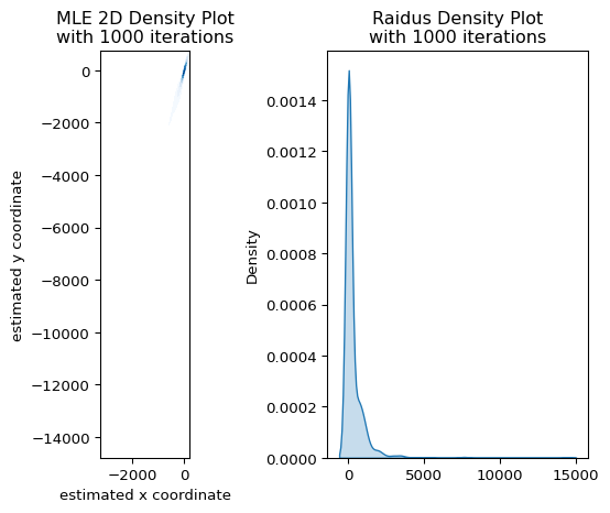
▶ Regression with MLE
\(\eqref{#eq-circle}\) に則り,もっと直接的に
\[
L(\beta) = (\sqrt{(x_i - \beta_1)^2 + (y_i - \beta_2)^2} - \beta_0)^2
\]
を最小する形でパラメーターを推定してみます.このとき.residualが\(N(0, \sigma)\) に従うならばLikelihoodは
\[
f(X_i\vert \beta, \sigma) = \frac{1}{\sqrt{2\pi}\sigma}\exp\left(-\frac{L(\beta)}{2\sigma^2}\right)
\]
と表せるので,これを用いて解いてみます.
コード
import numpy as npfrom scipy.optimize import minimizedef lik(parameters, x, y):= parameters[0 ]= parameters[1 ]= parameters[2 ]= parameters[3 ]= (np.sqrt((np.sqrt((x - x_0) ** 2 + (y - y_0) ** 2 ) - r_0)** 2 )) ** 2 = len (x) / 2 * np.log(sigma** 2 ) + 1 / (2 * sigma** 2 ) * np.sum (g_x)return Ldef mle_solver(tuple [str ] = ("x_coordinate" , "y_coordinate" )= df[xy_columns[0 ]].values= df[xy_columns[1 ]].values= minimize(lambda params: lik(params, x_attack, y_attack),1 , 1 , 20 , 1 ]),= "L-BFGS-B" ,return lik_model["x" ]= estimator_simulator(mle_solver)# plot = plt.subplots(1 , 2 )= mle_res[:, 0 ], y= mle_res[:, 1 ], cmap= "Blues" , fill= True , ax= axes[0 ])= mle_res[:, 2 ], cmap= "Blues" , fill= True , ax= axes[1 ])# Show the plot 0 ].set_xlabel("estimated x coordinate" )0 ].set_ylabel("estimated y coordinate" )0 ].set_title("MLE 2D Density Plot \n with 1000 iterations" )0 ].set_aspect("equal" )1 ].set_title("Raidus Density Plot \n with 1000 iterations" )
定式化は正しいはずですが,\((x_0, y_0, r_0)\) は効率的な推定量となっていない疑いがあることが読み取れます.
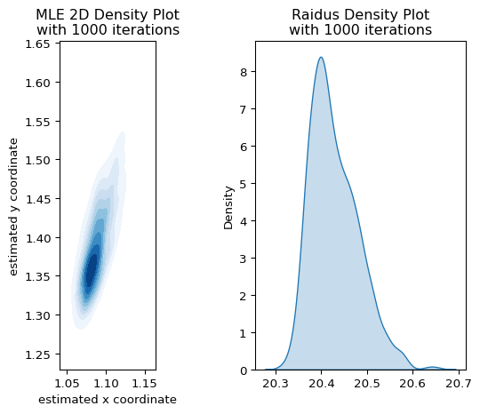
次に,
\[
L(\beta) = \sqrt{(x_i - \beta_1)^2 + (y_i - \beta_2)^2 - \beta_0^2} \label{#eq-mle}
\]
をLoss functionとして推定してみます.
コード
import numpy as npfrom scipy.optimize import minimizedef lik(parameters, x, y):= parameters[0 ]= parameters[1 ]= parameters[2 ]= parameters[3 ]= (x - x_0) ** 2 + (y - y_0) ** 2 - r_0** 2 = len (x) / 2 * np.log(sigma** 2 ) + 1 / (2 * sigma** 2 ) * np.sum (g_x)return Ldef mle_solver(tuple [str ] = ("x_coordinate" , "y_coordinate" )= df[xy_columns[0 ]].values= df[xy_columns[1 ]].values= minimize(lambda params: lik(params, x_attack, y_attack),1 , 1 , 20 , 1 ]),= "L-BFGS-B" ,return lik_model["x" ]= estimator_simulator(mle_solver)# plot = plt.subplots(1 , 2 )= mle_res[:, 0 ], y= mle_res[:, 1 ], cmap= "Blues" , fill= True , ax= axes[0 ])= mle_res[:, 2 ], cmap= "Blues" , fill= True , ax= axes[1 ])# Show the plot 0 ].set_xlabel("estimated x coordinate" )0 ].set_ylabel("estimated y coordinate" )0 ].set_title("MLE 2D Density Plot \n with 1000 iterations" )0 ].set_aspect("equal" )1 ].set_title("Raidus Density Plot \n with 1000 iterations" )
先程よりは精度良く推定できているように見えますが,\(\eqref{#eq-mle}\) は
\[
L(\beta) = \sqrt{\epsilon_i^2 + 2\beta_0 \epsilon_i}
\]
となるので,そもそもMLEの定式化が間違っていることがわかります.また,\(\beta_0\) が大きいほどresidualが大きくなる傾向があることから,unbiasedな推定量は得られていないことがわかります.
▶ Regression with stan
cmdstanを用いて砲台座標を推定する例を紹介します.まずstan modelを以下のように設定します.
砲撃距離のノイズについて \(N(0, 1)\) であることが既にわかっている状況を想定
予定砲撃距離 \(r_0\) は \(\operatorname{Uniform}(2, 30)\) の事前分布がある
data {int <lower =1 > N; // Number of data points array [N] real y; // outcomes array [N] real x; // outcomes parameters {real <lower =0 > r_0; // probability of success real x_0; // Center x-coordinate real y_0; // Center y-coordinate model {// priors 2 , 30 );real sigma = 1 ;// objective loss array [N] real circle_equation;for (i in 1 :N) {2 + (y[i] - y_0)^2 ) - r_0;0 , sigma);その後,このモデルを用いて推定したものが以下となります.
from cmdstanpy import CmdStanModel= gpd_dataframe(0 , 0 , 1 )= {"N" : df_stan.shape[0 ],"y" : df_stan.y_coordinate.values,"x" : df_stan.x_coordinate.values,"sigma" : 1 ,= CmdStanModel(stan_file= "./stanmodel.stan" )= model.sample(data= data, seed= 42 )
15:28:03 - cmdstanpy - INFO - compiling stan file /home/runner/work/regmonkey-datascience-blog/regmonkey-datascience-blog/posts/2025-03-02-find-coordinates/stanmodel.stan to exe file /home/runner/work/regmonkey-datascience-blog/regmonkey-datascience-blog/posts/2025-03-02-find-coordinates/stanmodel
15:28:11 - cmdstanpy - INFO - compiled model executable: /home/runner/work/regmonkey-datascience-blog/regmonkey-datascience-blog/posts/2025-03-02-find-coordinates/stanmodel
15:28:11 - cmdstanpy - INFO - CmdStan start processing
15:28:13 - cmdstanpy - INFO - CmdStan done processing.
15:28:13 - cmdstanpy - WARNING - Some chains may have failed to converge.
    Chain 1 had 310 divergent transitions (31.0%)
    Chain 2 had 341 divergent transitions (34.1%)
    Chain 3 had 293 divergent transitions (29.3%)
    Chain 4 had 320 divergent transitions (32.0%)
    Use the "diagnose()" method on the CmdStanMCMC object to see further information.
lp__
-22.627700
0.044144
1.21901
0.873056
-25.04740
-22.267300
-21.44630
886.907
1292.320
386.6200
1.00150
r_0
20.167700
0.429917
6.21166
7.274600
9.15980
20.889900
29.01690
208.133
258.641
90.7294
1.01911
x_0
0.151580
0.131551
1.88887
1.973320
-3.05708
0.195962
3.10467
199.727
234.533
87.0648
1.02554
y_0
-0.299075
0.419656
6.11452
7.154330
-8.93022
-1.015920
10.49840
220.608
278.533
96.1675
1.01959
Credible intervalを見ると \((0, 0)\) は推定区間に含まれている一方,Mean, Medianともに \(y_0\) の方は乖離した値が推定されてしまっています.