代表的なカーネル関数 – regmonkey datascience blog

代表的なカーネル

カーネル関数例

\[ \begin{align} \text{Gaussian kernel: } & k(u) = \frac{1}{\sqrt{2\pi}}\exp\left(-\frac{u^2}{2}\right)\\ \text{Epanechnikov kernel: } & k(u) = \frac{3}{4}(1 - u^2)\mathbf I\{|u| \leq 1\} = \frac{3}{4}\max\{1 - u^2, 0\}\\ \text{Biweight kernel: } & k(u) = \frac{15}{16}(1 - u^2)^2\mathbf I\{|u| \leq 1\}\\ \text{Uniform kernel: } & k(u) = \frac{1}{2}\mathbf I\{|u| \leq 1\}\\[5pt] \text{Triangular kernel: } & k(u) = (1 - |u|)\mathbf I\{|u| \leq 1\} \end{align} \]

上記のカーネル関数は以下のような特徴があります

\(K(u)\) is symmetric
\(\int k(u)du = 1\): KDEで推定された関数が密度関数であるための必要条件
\(\lim_{u\to\infty}k(u) = \lim_{u\to-\infty}k(u) = 0\)

カーネル関数別の密度関数推定結果の可視化

カーネル密度関数推定量を

\[ \hat f(x) = \frac{1}{nh}\sum_{i=1}^n k\left(\frac{X_i - x}{h}\right) \]

として，それぞれのカーネル関数を用いた推定結果を以下可視化します．

Code

import numpy as np
import matplotlib.pyplot as plt
import seaborn as sns
from sklearn.neighbors import KernelDensity

# okabe-ito color
color = [
    "#E69F00",
    "#56B4E9",
    "#009E73",
    "#F0E442",
    "#0072B2",
    "#D55E00",
    "#CC79A7",
    "#000000",
]


# Gaussian kernel function
def gaussian_kernel(u):
    return (1 / np.sqrt(2 * np.pi)) * np.exp(-0.5 * u**2)


def epanechnikov_kernel(u):
    const = 3 / 4
    return const * (1 - u**2) * (np.abs(u) <= 1).astype(float)


def biweight_kernel(u):
    const = 15 / 16
    return const * ((1 - u**2) ** 2) * (np.abs(u) <= 1).astype(float)


def uniform_kernel(u):
    return 0.5 * (np.abs(u) <= 1).astype(float)


def triangular_kernel(u):
    return (1 - np.abs(u)) * (np.abs(u) <= 1).astype(float)


# KDE
def kde(x, data, bandwidth, kernel_func):
    n = len(data)
    return (1 / (n * bandwidth)) * np.sum(kernel_func((x - data) / bandwidth))


# Load Old Faithful dataset (from seaborn)
data = sns.load_dataset("geyser")  # modern version of faithful dataset
waiting = data["waiting"].dropna().values

# Plot kernels
u = np.linspace(-3, 3, 200)
x_plot = np.linspace(40, 100, 1000)
fig, axes = plt.subplots(5, 2, figsize=(16, 6 * 5))

# gaussian
kde_vals = list(map(lambda x: kde(x, waiting, 0.5, gaussian_kernel), x_plot))
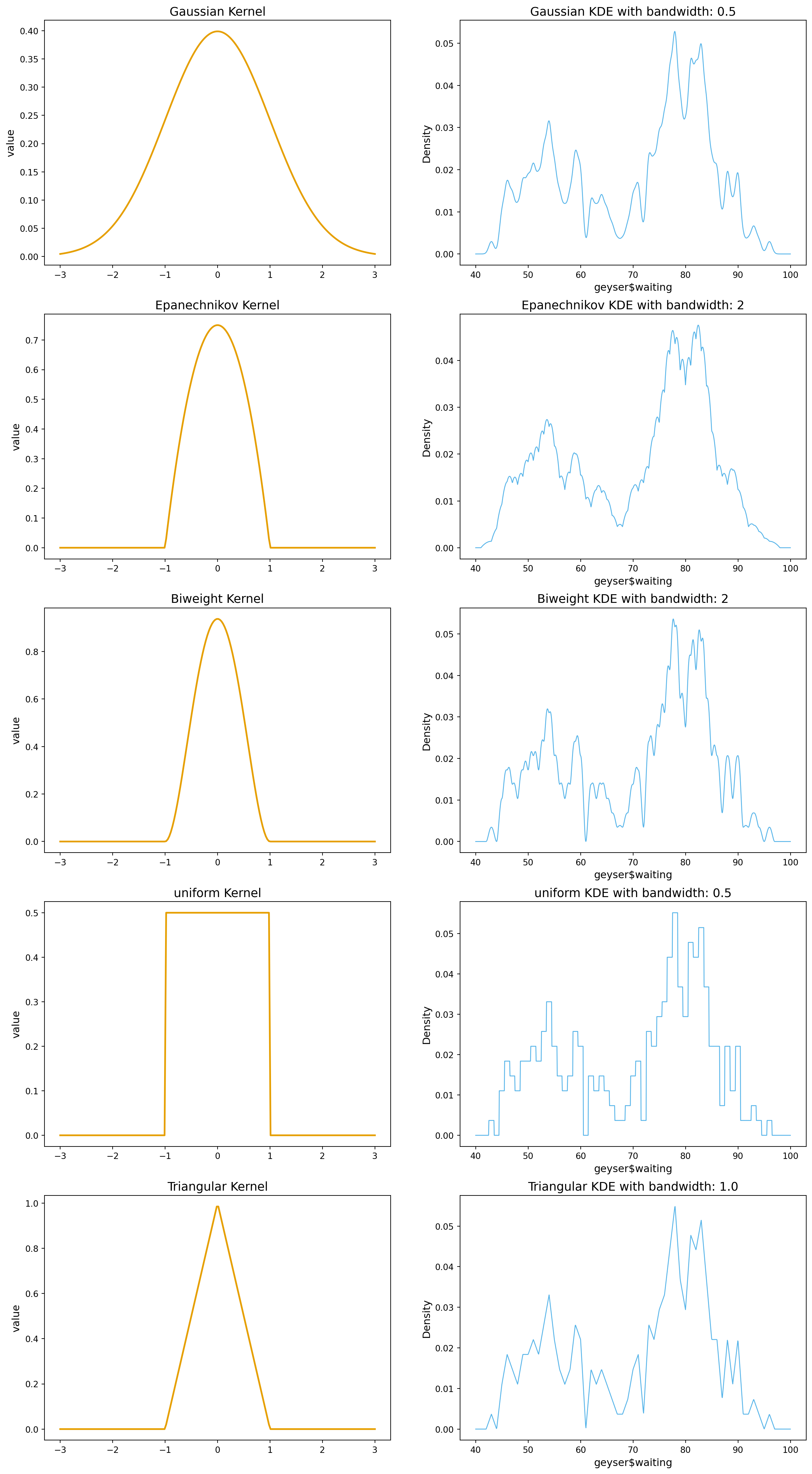
axes[0, 0].plot(u, gaussian_kernel(u), color[0], lw=2)
axes[0, 0].set_ylabel("value", fontsize=12)
axes[0, 0].set_title("Gaussian Kernel", fontsize=14)
axes[0, 1].plot(x_plot, kde_vals, color[1], lw=1)
axes[0, 1].set_ylabel("Density", fontsize=12)
axes[0, 1].set_xlabel("geyser$waiting", fontsize=12)
axes[0, 1].set_title("Gaussian KDE with bandwidth: 0.5", fontsize=14)


# epanechnikov
kde_vals = list(map(lambda x: kde(x, waiting, 2, epanechnikov_kernel), x_plot))
axes[1, 0].plot(u, epanechnikov_kernel(u), color[0], lw=2)
axes[1, 0].set_ylabel("value", fontsize=12)
axes[1, 0].set_title("Epanechnikov Kernel", fontsize=14)
axes[1, 1].plot(x_plot, kde_vals, color[1], lw=1)
axes[1, 1].set_ylabel("Density", fontsize=12)
axes[1, 1].set_xlabel("geyser$waiting", fontsize=12)
axes[1, 1].set_title("Epanechnikov KDE with bandwidth: 2", fontsize=14)

# Biweight
kde_vals = list(map(lambda x: kde(x, waiting, 1, biweight_kernel), x_plot))
axes[2, 0].plot(u, biweight_kernel(u), color[0], lw=2)
axes[2, 0].set_ylabel("value", fontsize=12)
axes[2, 0].set_title("Biweight Kernel", fontsize=14)
axes[2, 1].plot(x_plot, kde_vals, color[1], lw=1)
axes[2, 1].set_ylabel("Density", fontsize=12)
axes[2, 1].set_xlabel("geyser$waiting", fontsize=12)
axes[2, 1].set_title("Biweight KDE with bandwidth: 2", fontsize=14)

# Uniform
kde_vals = list(map(lambda x: kde(x, waiting, 0.5, uniform_kernel), x_plot))
axes[3, 0].plot(u, uniform_kernel(u), color[0], lw=2)
axes[3, 0].set_ylabel("value", fontsize=12)
axes[3, 0].set_title("uniform Kernel", fontsize=14)
axes[3, 1].plot(x_plot, kde_vals, color[1], lw=1)
axes[3, 1].set_ylabel("Density", fontsize=12)
axes[3, 1].set_xlabel("geyser$waiting", fontsize=12)
axes[3, 1].set_title("uniform KDE with bandwidth: 0.5", fontsize=14)

# Triangular
kde_vals = list(map(lambda x: kde(x, waiting, 1.0, triangular_kernel), x_plot))
axes[4, 0].plot(u, triangular_kernel(u), color[0], lw=2)
axes[4, 0].set_ylabel("value", fontsize=12)
axes[4, 0].set_title("Triangular Kernel", fontsize=14)
axes[4, 1].plot(x_plot, kde_vals, color[1], lw=1)
axes[4, 1].set_ylabel("Density", fontsize=12)
axes[4, 1].set_xlabel("geyser$waiting", fontsize=12)
axes[4, 1].set_title("Triangular KDE with bandwidth: 1.0", fontsize=14)

plt.show()