中年男性の中性脂肪分布はLognormalで近似できるか?

統計
python
Author

Ryo Nakagami

Published

2025-12-15

Modified

2025-12-17

1. リサーチクエッション

  • アメリカの中年男性(40-59歳)の血中中性脂肪(トリグリセリド)濃度は,Lognormal分布でどの程度近似できるか?

背景

血中脂質値は多くの場合,正規分布ではなく右に歪んだ分布を示す。特に中性脂肪は,生活習慣や遺伝的要因により極端な高値を示す個人が存在するため,Lognormal分布での近似がしばしば用いられます. このノートでは,米国の代表的な健康調査データを用いて,この仮説を検証したいとおもいます.

2. Data

データソース

使用ファイル

ファイル 内容
DEMO_L.xpt 人口統計学的データ(年齢,性別等)
TRIGLY_L.xpt 中性脂肪・LDLコレステロールデータ

対象者の選択基準

  1. 性別: 男性 (RIAGENDR = 1)
  2. 年齢: 40-59歳 (RIDAGEYR)
  3. 中性脂肪データ: 欠損なし (LBXTLG is not null)
  4. サンプルウェイト: 有効 (WTSAF2YR > 0)

測定方法

  • 中性脂肪(Triglycerides)は,12歳以上の参加者のうち,8-24時間絶食という空腹条件を満たした部分標本(fasting subsample) に対してのみ測定

サンプルウェイト

  • WTSAF2YR(空腹時サブサンプル2年MEC重み)を使用
  • see here

Definition 1 WTSAF2YR

  • 「当該参加者が米国の民間非施設居住人口の何人規模のグループをを代表しているか」を表す設計ウェイト
  • ある参加者のWTSAF2YR = 50,000 の場合,その参加者は母集団内の約50,000人グループを代表することを意味する

ウェイトの基本的な考えは

\[ \text{sample person's weight} = \frac{1}{\text{probability of selection}} \]

詳しい説明は省略しますが,

Four Stages of NHANES Sampling Procedure
  1. 米国全体を分割した一次抽出(PSU:郡または郡群)
  2. 選ばれた PSU 内で小地域(街区・セグメント)が選ばれる
  3. 選ばれたセグメント内で,世帯(household) が抽出される
  4. 世帯内の構成員のうち,調査対象者として個人が選ばれる

という流れでNHANESでは層化抽出が行われ probability of selection が定まります.解釈としては

“A sample weight is assigned to each sample person. It is a measure of the number of people in the population represented by that sample person in NHANES, reflecting the unequal probability of selection, an adjustment for sample person non-response, and adjustment to account for differences between the final sample and the total population based on independent population control totals.”

したがって,母集団平均の推定には

\[ \text{weighted mean} = \frac{\sum \text{WTSAF2YR} \times \text{value}}{\sum \text{WTSAF2YR}} \]

となります.

3. 分析方針

Lognormal分布の仮定

血中中性脂肪濃度は以下の特徴を持つため,Lognormal分布での近似をおこないます:

  1. 正の値のみ: 濃度は必ず正の値をとる
  2. 右に歪んだ分布: 極端な高値を示す個人が存在
  3. 乗法的な影響: 遺伝・食事・運動などの要因が乗法的に作用すると仮定

適合度の評価方法

評価方法 目的 判断
重み付きヒストグラム vs PDF 視覚的な分布形状の比較 主観的判断
Q-Qプロット 分位点の一致度を評価 主観的判断
Kolmogorov-Smirnov検定 統計的な適合度検定 統計的判定

4. 推定関数

重み付きQQ plot

Code
import numpy as np

def weighted_quantiles(
    values: np.ndarray, weights: np.ndarray, quantiles: np.ndarray
) -> np.ndarray:
    """
    Compute weighted quantiles.

    Parameters
    ----------
    values : array-like
        Array of observed values.
    weights : array-like
        Sample weights corresponding to each observation.
    quantiles : array-like
        Quantiles to compute (values between 0 and 1).

    Returns
    -------
    ndarray
        Values corresponding to the specified quantiles.
    """
    sorted_indices = np.argsort(values)
    sorted_values = values[sorted_indices]
    sorted_weights = weights[sorted_indices]

    # Cumulative sum of weights, normalized to [0, 1]
    cumsum_normalized = np.cumsum(sorted_weights) / np.sum(sorted_weights)

    return np.interp(quantiles, cumsum_normalized, sorted_values)

重み付きKS検定の実装

  • scipy の ks_2samp をベースに、両側からのCDF差を計算する方法を採用
  • effective sample sizeは \((\sum w_i)^2 / \sum w_i^2\) で計算 (see Monahan, J. (2011). Numerical Methods of Statistics.)
Code
from typing import Callable
from scipy import stats

def weighted_ks_1samp(
    values: np.ndarray, weights: np.ndarray, cdf_func: Callable[[np.ndarray], np.ndarray]
) -> tuple[float, float]:
    """
    Perform a one-sample weighted Kolmogorov–Smirnov test.

    The p-value is computed using an effective sample size
    (Kish's effective sample size), following the approach
    proposed by Monahan.

    Parameters
    ----------
    values : np.ndarray
        Array of observed values.
    weights : np.ndarray
        Sample weights corresponding to each observation.
    cdf_func : Callable[[np.ndarray], np.ndarray]
        CDF function of the theoretical distribution. It takes
        an array of values and returns cumulative probabilities.

    Returns
    -------
    tuple[float, float]
        (ks_stat, p_value) – the KS statistic and the asymptotic p-value.

    References
    ----------
    Monahan, J. (2011). *Numerical Methods of Statistics*.
    """
    sorted_indices = np.argsort(values)
    sorted_values = values[sorted_indices]
    sorted_weights = weights[sorted_indices]

    # Weighted ECDF: F_n(x) = Σ w_i * I(X_i ≤ x) / Σ w_i
    cumsum = np.cumsum(sorted_weights)
    total_weight = cumsum[-1]
    ecdf_after = cumsum / total_weight          # F_n(x) = P(X ≤ x)
    ecdf_before = np.concatenate([[0], ecdf_after[:-1]])  # F_n(x−)

    # Theoretical CDF
    theoretical_cdf = cdf_func(sorted_values)

    # KS statistic: maximum deviation from both sides
    d_plus = np.max(ecdf_after - theoretical_cdf)    # sup(F_n − F)
    d_minus = np.max(theoretical_cdf - ecdf_before)  # sup(F − F_n)
    ks_stat = max(d_plus, d_minus)

    # Effective sample size (Kish's effective sample size)
    n_eff = total_weight**2 / np.sum(sorted_weights**2)

    # Asymptotic p-value (Kolmogorov distribution)
    p_value = stats.kstwobign.sf(np.sqrt(n_eff) * ks_stat)

    return float(ks_stat), float(np.clip(p_value, 0, 1))

5. 分析コード

Code
"""
NHANES August 2021-August 2023 中年男性の中性脂肪分析
ヒストグラムとlognormal分布の比較
(サンプルウェイト WTSAF2YR を考慮)
"""

import polars as pl
import pyreadstat
import matplotlib.pyplot as plt


def load_data():
    """DEMO_L と TRIGLY_L データを読み込み結合"""
    demo_pd, _ = pyreadstat.read_xport("DEMO_L.xpt", encoding="latin1")
    trigly_pd, _ = pyreadstat.read_xport("TRIGLY_L.xpt", encoding="latin1")

    demo = pl.from_pandas(demo_pd)
    trigly = pl.from_pandas(trigly_pd)

    df = demo.join(trigly, on="SEQN", how="inner")
    return df


def filter_middle_aged_men(df: pl.DataFrame) -> pl.DataFrame:
    """
    中年男性(40-59歳)をフィルタリング
    - RIAGENDR: 1 = Male
    - RIDAGEYR: 年齢
    - LBXTLG: 中性脂肪 (mg/dL)
    - WTSAF2YR > 0: 有効なサンプルウェイトを持つ参加者のみ
    """
    filtered = df.filter(
        (pl.col("RIAGENDR") == 1)
        & (pl.col("RIDAGEYR") >= 40)
        & (pl.col("RIDAGEYR") <= 59)
        & (pl.col("LBXTLG").is_not_null())
        & (pl.col("WTSAF2YR") > 0)
    )
    return filtered


def weighted_mean(values: np.ndarray, weights: np.ndarray) -> float:
    """重み付き平均"""
    return np.sum(values * weights) / np.sum(weights)


def weighted_std(values: np.ndarray, weights: np.ndarray) -> float:
    """重み付き標準偏差"""
    mean = weighted_mean(values, weights)
    variance = np.sum(weights * (values - mean) ** 2) / np.sum(weights)
    return np.sqrt(variance)


def weighted_median(values: np.ndarray, weights: np.ndarray) -> float:
    """重み付き中央値"""
    sorted_indices = np.argsort(values)
    sorted_values = values[sorted_indices]
    sorted_weights = weights[sorted_indices]
    cumsum = np.cumsum(sorted_weights)
    cutoff = np.sum(sorted_weights) / 2.0
    return sorted_values[np.searchsorted(cumsum, cutoff)]


def weighted_histogram(values: np.ndarray, weights: np.ndarray, bins: int = 50):
    """重み付きヒストグラムのデータを計算"""
    hist, bin_edges = np.histogram(values, bins=bins, weights=weights, density=True)
    return hist, bin_edges


def weighted_ecdf(values: np.ndarray, weights: np.ndarray) -> tuple:
    """重み付き経験累積分布関数を計算"""
    sorted_indices = np.argsort(values)
    sorted_values = values[sorted_indices]
    sorted_weights = weights[sorted_indices]

    cumsum = np.cumsum(sorted_weights)
    ecdf = cumsum / cumsum[-1]

    return sorted_values, ecdf


def filter_by_percentile(
    values: np.ndarray,
    weights: np.ndarray,
    lower_pct: float = 0.05,
    upper_pct: float = 0.95,
) -> tuple[np.ndarray, np.ndarray]:
    """
    重み付きパーセンタイルでデータをフィルタリング

    Parameters
    ----------
    values : np.ndarray
        観測値
    weights : np.ndarray
        サンプルウェイト
    lower_pct : float
        下限パーセンタイル(0-1)
    upper_pct : float
        上限パーセンタイル(0-1)

    Returns
    -------
    filtered_values : np.ndarray
        フィルタリング後の観測値
    filtered_weights : np.ndarray
        フィルタリング後のウェイト
    """
    quantile_bounds = weighted_quantiles(values, weights, np.array([lower_pct, upper_pct]))
    lower_bound, upper_bound = quantile_bounds[0], quantile_bounds[1]

    mask = (values >= lower_bound) & (values <= upper_bound)
    return values[mask], weights[mask], lower_bound, upper_bound


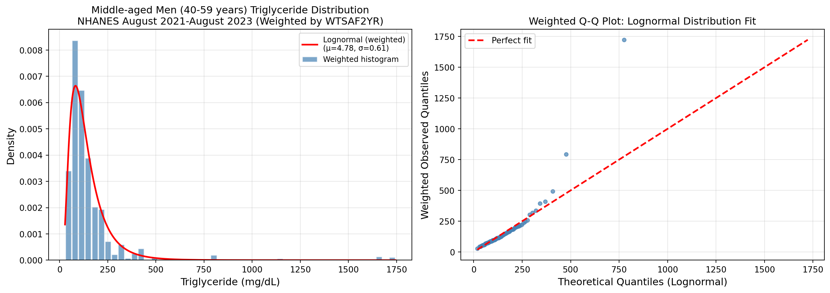
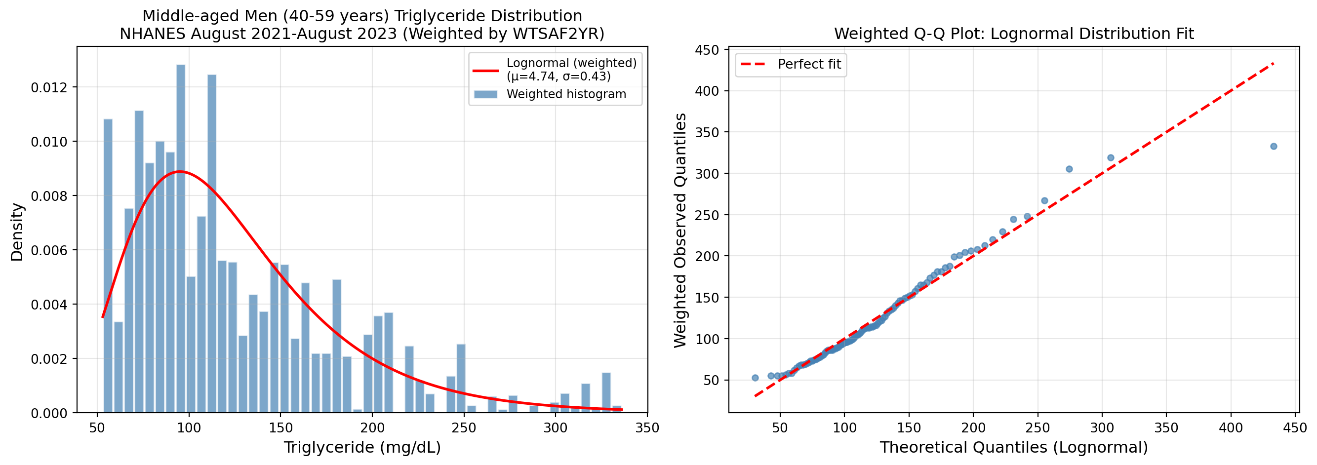
def analyze_and_plot(
    triglyceride_values: np.ndarray,
    weights: np.ndarray,
    save_suffix: str = "",
):
    """ヒストグラムとlognormal分布の比較プロット(重み付き)"""

    # --- 重み付きパラメータ推定 ---
    log_values = np.log(triglyceride_values)
    mu_weighted = weighted_mean(log_values, weights)
    sigma_weighted = weighted_std(log_values, weights)

    # プロット作成
    fig, axes = plt.subplots(1, 2, figsize=(14, 5))

    # --- 左: ヒストグラムとlognormal PDF ---
    ax1 = axes[0]

    # 重み付きヒストグラム
    hist, bin_edges = weighted_histogram(triglyceride_values, weights, bins=50)
    bin_centers = (bin_edges[:-1] + bin_edges[1:]) / 2
    bin_width = bin_edges[1] - bin_edges[0]
    ax1.bar(
        bin_centers,
        hist,
        width=bin_width * 0.9,
        alpha=0.7,
        color="steelblue",
        edgecolor="white",
        label="Weighted histogram",
    )

    # Lognormal PDF(重み付きパラメータ)
    x = np.linspace(triglyceride_values.min(), triglyceride_values.max(), 500)
    pdf_weighted = stats.lognorm.pdf(x, s=sigma_weighted, scale=np.exp(mu_weighted))
    ax1.plot(
        x,
        pdf_weighted,
        "r-",
        linewidth=2,
        label=f"Lognormal (weighted)\n(μ={mu_weighted:.2f}, σ={sigma_weighted:.2f})",
    )

    ax1.set_xlabel("Triglyceride (mg/dL)", fontsize=12)
    ax1.set_ylabel("Density", fontsize=12)
    ax1.set_title(
        "Middle-aged Men (40-59 years) Triglyceride Distribution\n"
        "NHANES August 2021-August 2023 (Weighted by WTSAF2YR)",
        fontsize=12,
    )
    ax1.legend(fontsize=9)
    ax1.grid(True, alpha=0.3)

    # --- 右: 重み付きQ-Qプロット ---
    ax2 = axes[1]

    # 重み付き分位点を計算
    n_quantiles = 100  # プロット用の分位点数
    prob_points = np.linspace(0.001, 0.999, n_quantiles)  # 0.1%〜99.9%で裾もカバー

    # 重み付き観測分位点
    observed_quantiles = weighted_quantiles(triglyceride_values, weights, prob_points)

    # 理論分位点(Lognormal)
    theoretical_quantiles = stats.lognorm.ppf(
        prob_points, s=sigma_weighted, scale=np.exp(mu_weighted)
    )

    ax2.scatter(
        theoretical_quantiles, observed_quantiles, alpha=0.7, s=20, c="steelblue"
    )
    min_val = min(theoretical_quantiles.min(), observed_quantiles.min())
    max_val = max(theoretical_quantiles.max(), observed_quantiles.max())
    ax2.plot(
        [min_val, max_val], [min_val, max_val], "r--", linewidth=2, label="Perfect fit"
    )

    ax2.set_xlabel("Theoretical Quantiles (Lognormal)", fontsize=12)
    ax2.set_ylabel("Weighted Observed Quantiles", fontsize=12)
    ax2.set_title("Weighted Q-Q Plot: Lognormal Distribution Fit", fontsize=12)
    ax2.legend(fontsize=10)
    ax2.grid(True, alpha=0.3)

    plt.tight_layout()
    plt.savefig(f"triglyceride_analysis{save_suffix}.png", dpi=150, bbox_inches="tight")
    plt.show()

    # 統計情報を出力
    print("\n" + "=" * 70)
    print("Statistics: Middle-aged Men (40-59 years) Triglyceride")
    print("NHANES August 2021-August 2023 (with sample weights)")
    print("=" * 70)
    print(f"Sample size (n): {len(triglyceride_values)}")
    print(f"Sum of weights: {np.sum(weights):,.0f}")

    print(f"\n[Descriptive Statistics - WEIGHTED (population estimates)]")
    print(f"  Mean: {weighted_mean(triglyceride_values, weights):.1f} mg/dL")
    print(f"  Median: {weighted_median(triglyceride_values, weights):.1f} mg/dL")
    print(f"  Std Dev: {weighted_std(triglyceride_values, weights):.1f} mg/dL")

    print(f"\n[Descriptive Statistics - UNWEIGHTED (sample only)]")
    print(f"  Mean: {np.mean(triglyceride_values):.1f} mg/dL")
    print(f"  Median: {np.median(triglyceride_values):.1f} mg/dL")
    print(f"  Std Dev: {np.std(triglyceride_values, ddof=1):.1f} mg/dL")
    print(f"  Min: {np.min(triglyceride_values):.1f} mg/dL")
    print(f"  Max: {np.max(triglyceride_values):.1f} mg/dL")

    print(f"\n[Lognormal Parameters - WEIGHTED]")
    print(f"  μ (log-scale mean): {mu_weighted:.4f}")
    print(f"  σ (log-scale std): {sigma_weighted:.4f}")
    print(f"  Median from fit (exp(μ)): {np.exp(mu_weighted):.1f} mg/dL")


    # 適合度検定 (Kolmogorov-Smirnov)
    def cdf_func(x):
        return stats.lognorm.cdf(x, s=sigma_weighted, scale=np.exp(mu_weighted))

    # 重み付きKS検定
    ks_stat_weighted, ks_pvalue_weighted = weighted_ks_1samp(
        triglyceride_values, weights, cdf_func
    )

    # 有効サンプルサイズ(Kish's effective sample size)
    n_eff = (np.sum(weights) ** 2) / np.sum(weights**2)

    # 重みなしKS検定(参考)
    ks_stat_unweighted, ks_pvalue_unweighted = stats.kstest(
        triglyceride_values, cdf_func
    )

    print("\n[Goodness-of-fit (Kolmogorov-Smirnov)]")
    print("  [WEIGHTED]")
    print(f"    KS statistic: {ks_stat_weighted:.4f}")
    print(f"    Asymptotic p-value: {ks_pvalue_weighted:.4f}")
    print(f"    Effective sample size (Kish): {n_eff:.1f}")
    print("    Note: p-value uses asymptotic approximation with n_eff")
    if ks_pvalue_weighted > 0.05:
        print("    -> p > 0.05: No significant difference from lognormal")
    else:
        print("    -> p < 0.05: Significantly different from lognormal")

    print("  [UNWEIGHTED (reference)]")
    print(f"    KS statistic: {ks_stat_unweighted:.4f}")
    print(f"    p-value: {ks_pvalue_unweighted:.4f}")
    if ks_pvalue_unweighted > 0.05:
        print("    -> p > 0.05: No significant difference from lognormal")
    else:
        print("    -> p < 0.05: Significantly different from lognormal")
    print("=" * 70)


def main():
    print("Loading NHANES data...")
    df = load_data()

    print("Filtering middle-aged men (40-59 years) with valid weights...")
    middle_aged_men = filter_middle_aged_men(df)

    triglyceride_values = middle_aged_men.select("LBXTLG").to_numpy().flatten()
    weights = middle_aged_men.select("WTSAF2YR").to_numpy().flatten()

    print(f"Sample size: {len(triglyceride_values)}")
    print(f"Excluded (WTSAF2YR = 0 or missing): checked")

    analyze_and_plot(triglyceride_values, weights)

if __name__ == "__main__":
    main()
Loading NHANES data...
Filtering middle-aged men (40-59 years) with valid weights...
Sample size: 362
Excluded (WTSAF2YR = 0 or missing): checked


======================================================================
Statistics: Middle-aged Men (40-59 years) Triglyceride
NHANES August 2021-August 2023 (with sample weights)
======================================================================
Sample size (n): 362
Sum of weights: 39,758,496

[Descriptive Statistics - WEIGHTED (population estimates)]
  Mean: 152.6 mg/dL
  Median: 111.0 mg/dL
  Std Dev: 180.6 mg/dL

[Descriptive Statistics - UNWEIGHTED (sample only)]
  Mean: 149.9 mg/dL
  Median: 108.5 mg/dL
  Std Dev: 160.2 mg/dL
  Min: 28.0 mg/dL
  Max: 1745.0 mg/dL

[Lognormal Parameters - WEIGHTED]
  μ (log-scale mean): 4.7800
  σ (log-scale std): 0.6062
  Median from fit (exp(μ)): 119.1 mg/dL

[Goodness-of-fit (Kolmogorov-Smirnov)]
  [WEIGHTED]
    KS statistic: 0.0893
    Asymptotic p-value: 0.0344
    Effective sample size (Kish): 254.8
    Note: p-value uses asymptotic approximation with n_eff
    -> p < 0.05: Significantly different from lognormal
  [UNWEIGHTED (reference)]
    KS statistic: 0.0892
    p-value: 0.0059
    -> p < 0.05: Significantly different from lognormal
======================================================================

6. 結果解釈

QQ plot

観測点の位置 意味
直線上 理論分布と一致
直線より上 観測データの裾が厚い (heavy tail)
直線より下 観測データの裾が薄い (light tail)

今回のデータの特徴

領域 観察されたパターン 解釈
下側の裾(低値) ほぼ直線上 Lognormalと良く一致
中央部(50-300 mg/dL) 直線上 良好なフィット
上側の裾(高値) 直線より上に乖離 Lognormalより裾が厚い

Insights

  1. 全体的なフィット: Lognormal分布は中性脂肪分布の大部分(約95%)を良く近似する
  2. 上側の裾の逸脱: 極端な高値(概ね400 mg/dL以上)の出現頻度がLognormal分布の予測より高い
  3. 臨床的含意:
    • 高トリグリセリド血症の有病率推定において、Lognormalモデルは過小評価のリスクがある
    • リスク評価では、より裾の厚い分布(例:一般化ガンマ分布)の検討も有用かも?

7. 追加分析

Code
def additional_analysis():
    print("Loading NHANES data...")
    df = load_data()

    print("Filtering middle-aged men (40-59 years) with valid weights...")
    middle_aged_men = filter_middle_aged_men(df)

    triglyceride_values = middle_aged_men.select("LBXTLG").to_numpy().flatten()
    weights = middle_aged_men.select("WTSAF2YR").to_numpy().flatten()

    # === 5%-95%パーセンタイル範囲での分析 ===
    print("\n" + "=" * 70)
    print("ANALYSIS 2: Trimmed Data (5th-95th Percentile)")
    print("=" * 70)
    trimmed_values, trimmed_weights, lower_bound, upper_bound = filter_by_percentile(
        triglyceride_values, weights, lower_pct=0.05, upper_pct=0.95
    )
    print(f"Percentile range: [{lower_bound:.1f}, {upper_bound:.1f}] mg/dL")
    print(f"Trimmed sample size: {len(trimmed_values)} (from {len(triglyceride_values)})")
    print(f"Excluded: {len(triglyceride_values) - len(trimmed_values)} extreme values")

    analyze_and_plot(trimmed_values, trimmed_weights, save_suffix="_trimmed_5_95")

additional_analysis()
Loading NHANES data...
Filtering middle-aged men (40-59 years) with valid weights...

======================================================================
ANALYSIS 2: Trimmed Data (5th-95th Percentile)
======================================================================
Percentile range: [52.8, 351.4] mg/dL
Trimmed sample size: 326 (from 362)
Excluded: 36 extreme values


======================================================================
Statistics: Middle-aged Men (40-59 years) Triglyceride
NHANES August 2021-August 2023 (with sample weights)
======================================================================
Sample size (n): 326
Sum of weights: 35,785,691

[Descriptive Statistics - WEIGHTED (population estimates)]
  Mean: 126.0 mg/dL
  Median: 111.0 mg/dL
  Std Dev: 59.0 mg/dL

[Descriptive Statistics - UNWEIGHTED (sample only)]
  Mean: 127.4 mg/dL
  Median: 108.0 mg/dL
  Std Dev: 63.0 mg/dL
  Min: 53.0 mg/dL
  Max: 336.0 mg/dL

[Lognormal Parameters - WEIGHTED]
  μ (log-scale mean): 4.7400
  σ (log-scale std): 0.4308
  Median from fit (exp(μ)): 114.4 mg/dL

[Goodness-of-fit (Kolmogorov-Smirnov)]
  [WEIGHTED]
    KS statistic: 0.0688
    Asymptotic p-value: 0.2259
    Effective sample size (Kish): 230.1
    Note: p-value uses asymptotic approximation with n_eff
    -> p > 0.05: No significant difference from lognormal
  [UNWEIGHTED (reference)]
    KS statistic: 0.0704
    p-value: 0.0755
    -> p > 0.05: No significant difference from lognormal
======================================================================
Note追加分析解釈
  • log-scale が0.6062 → 0.0688に減少: 裾の極端な値を除外したことで分散が小さくなった
  • KS統計量も0.0893 → 0.4308に減少: 経験分布と理論分布の最大乖離が縮小
  • Q-Qプロットを見ても,トリミング後は理論直線(赤破線)にデータポイントがいい感じに乗っている.特に上側の裾の逸脱が解消
  • ただし,そもそも上位5%を異常値として除外できるかどうかは,適合度のみではわからない.
    • 分析目的などによりケースバイケースで判断が必要

Appendix: トリグリセリド

Definition 2 中性脂肪 / トリグリセリド

  • 肉や魚・食用油など食品中の脂質や,体内の脂質の大部分を占める物質
  • 中性脂肪は重要なエネルギー源であり,ビタミンの吸収を助けたり,必須脂肪酸(体内で合成されない脂肪酸)を摂取するという点においても不可欠なもの
  • とりすぎると体脂肪として蓄えられて肥満を招き,心筋梗塞などになりやすくなる
  • 血液中の中性脂肪値は特定健診の検査項目に含まれており,空腹時150mg/dⅬ以上,随時175mg/dⅬ以上になると「高TG(トリグリセライド)血症」とされる
測定項目 英語名 略称 単位 説明
総コレステロール Total Cholesterol TC mg/dL 血中コレステロールの総量.心血管疾患リスク評価の基本指標
高比重リポ蛋白コレステロール High-Density Lipoprotein Cholesterol HDL-C mg/dL いわゆる「善玉」コレステロール.高値は心血管リスク低下と関連
低比重リポ蛋白コレステロール Low-Density Lipoprotein Cholesterol LDL-C mg/dL いわゆる「悪玉」コレステロール.動脈硬化リスクと強く関連
中性脂肪 Triglycerides TG mg/dL 血中脂質の一種.エネルギー代謝やメタボリックリスクと関連

Appendix: QQ plot

データ解析のための数理統計入門ベースで行くとQQ plotは以下のように定義されています.

Definition 3 QQ plot

確率変数 \(X_1, \cdots, X_n \overset{\mathrm{iid}}{\sim} F\) とし,その順序統計量を

\[ X_{(1)} \leq \cdots \leq X_{(n)} \]

とする.\(X_{(j)}\) の実現値 \(x_{(j)}\) として, \(F\) の逆変換を施した点

\[ (x_{(j)}, F^{-1}(j/(n+1))) \]

をplotしたものをQQ plotという.

この定義を正とすると,分析におけるQQ plotはQQ plotではない.ただ,久保川先生では

\[ F(x_{(j)}, j/(n+1)) \]

をplotしたものをPP plotと呼んでおり,分析におけるQQ plotは久保川流でいくならば PP plotということになります.PP plotの理論的根拠は, 確率積分変換により \(F(X)\) は一様分布に従い,iid sampleは各点独立に

\[ \mathbb E[F(X_{(j)})] = \frac{j}{n+1} \]

になるはずという考えが背景にあります.

References