シグモイド基底関数とtanh基底関数の線形モデルの等価性

シグモイド関数とtanh関数

Definition 1 tanh関数

双曲線正接関数（hyperbolic tangent function）\(\begin{equation*}\tanh \left( x\right) :\mathbb{R} \rightarrow \mathbb{R} \end{equation*}\) の定義は以下

\[ \begin{eqnarray*}\tanh \left( x\right) &=&\frac{\sinh \left( x\right) }{\cosh \left( x\right) } \\ &=&\frac{\frac{e^{x}-e^{-x}}{2}}{\frac{e^{x}+e^{-x}}{2}} \\ &=&\frac{e^{x}-e^{-x}}{e^{x}+e^{-x}} \end{eqnarray*} \]

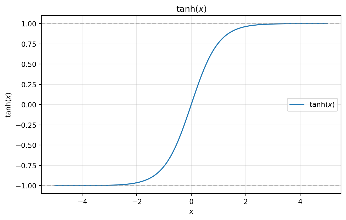
Example 1 tanh関数の形状

tanh関数のplot

import matplotlib.pyplot as plt
import numpy as np

x = np.linspace(-5, 5, 300)
y = np.tanh(x)

fig, ax = plt.subplots(figsize=(7, 4.5))
ax.plot(x, y, label=r"$\tanh(x)$")
ax.axhline(y=1, linestyle="--", color="gray", alpha=0.5)
ax.axhline(y=-1, linestyle="--", color="gray", alpha=0.5)
ax.set(xlabel="x", ylabel=r"$\tanh(x)$", title=r"$\tanh(x)$")
ax.legend()
ax.grid(True, alpha=0.3)
plt.tight_layout()
plt.show()

Theorem 1 シグモイド関数との関係

シグモイド関数

\[ \sigma(a) = \frac{1}{1 + \exp(-a)} \]

について，

\[ \tanh(a) = 2\sigma(2a) - 1 \]

Proof

\(\tanh(a)\) の分母・分子に \(\exp(a)\) を掛けると

\[ \begin{align} \tanh(a) &= \frac{\exp(2a) - 1}{\exp(2a) + 1}\\ &= \frac{2\exp(2a) - (\exp(2a) + 1)}{\exp(2a) + 1}\\ &= 2\frac{\exp(2a)}{\exp(2a) + 1} - 1\\ &= 2\frac{1}{1 + \exp(-2a)} - 1\\ &= 2\sigma(2a) - 1 \end{align} \]

Theorem 2 ロジスティクシグモイド関数とtanh線型結合関数の等価性

シグモイド基底関数による線形モデル

\[ y(\mathbf x, \mathbf w) = w_0 + \sum_{j=1}^{M} w_j \, \sigma\!\left(\frac{x - \mu_j}{s}\right) \]

と tanh 基底関数による線形モデル

\[ y(\mathbf x, \mathbf u) = u_0 + \sum_{j=1}^{M} u_j \, \tanh\!\left(\frac{x - \mu_j}{2s}\right) \]

は，以下のパラメータ変換により等価である：

\[ \begin{cases} u_0 = w_0 + \displaystyle\sum_{j=1}^{M} \frac{w_j}{2} \\[6pt] u_j = \dfrac{w_j}{2} \quad (j = 1, \dots, M) \end{cases} \]

Proof

\(\tanh(a) = 2\sigma(2a) - 1\) より \(\sigma(a) = \dfrac{1 + \tanh(a/2)}{2}\) が成り立つ。

これを \(a = \dfrac{x - \mu_j}{s}\) として代入すると

\[ \begin{align} y(\mathbf x, \mathbf w) &= w_0 + \sum_{j=1}^{M} w_j \, \sigma\!\left(\frac{x - \mu_j}{s}\right) \\ &= w_0 + \sum_{j=1}^{M} w_j \, \frac{1 + \tanh\!\left(\dfrac{x - \mu_j}{2s}\right)}{2} \\ &= w_0 + \sum_{j=1}^{M} \frac{w_j}{2} + \sum_{j=1}^{M} \frac{w_j}{2} \, \tanh\!\left(\frac{x - \mu_j}{2s}\right) \\ &= \underbrace{\left(w_0 + \sum_{j=1}^{M} \frac{w_j}{2}\right)}_{u_0} + \sum_{j=1}^{M} \underbrace{\frac{w_j}{2}}_{u_j} \, \tanh\!\left(\frac{x - \mu_j}{2s}\right) \end{align} \]

したがって \(u_0 = w_0 + \sum_{j=1}^{M} \frac{w_j}{2}\)，\(u_j = \frac{w_j}{2}\) と置けば両モデルは一致する。\(\blacksquare\)

Example 2 数値的な検証

等価性の数値検証

import matplotlib.pyplot as plt
import numpy as np


def sigmoid(a):
    return 1 / (1 + np.exp(-a))


# --- パラメータ設定 ---
M = 4
rng = np.random.default_rng(42)
w = rng.standard_normal(M + 1)          # w_0, w_1, ..., w_M
mu = np.linspace(-3, 3, M)
s = 1.0

# --- パラメータ変換 ---
u_0 = w[0] + np.sum(w[1:]) / 2
u_rest = w[1:] / 2

# --- モデル評価 ---
x = np.linspace(-6, 6, 500)

y_sigmoid = w[0] + sum(
    w[j + 1] * sigmoid((x - mu[j]) / s) for j in range(M)
)
y_tanh = u_0 + sum(
    u_rest[j] * np.tanh((x - mu[j]) / (2 * s)) for j in range(M)
)

# --- プロット ---
fig, ax = plt.subplots(figsize=(7, 4.5))
ax.plot(x, y_sigmoid, label=r"sigmoid model $y(\mathbf{x}, \mathbf{w})$")
ax.plot(x, y_tanh, linestyle="--", label=r"tanh model $y(\mathbf{x}, \mathbf{u})$")
ax.set(xlabel="x", ylabel="y", title="sigmoid basis vs tanh basis")
ax.legend()
ax.grid(True, alpha=0.3)
plt.tight_layout()
plt.show()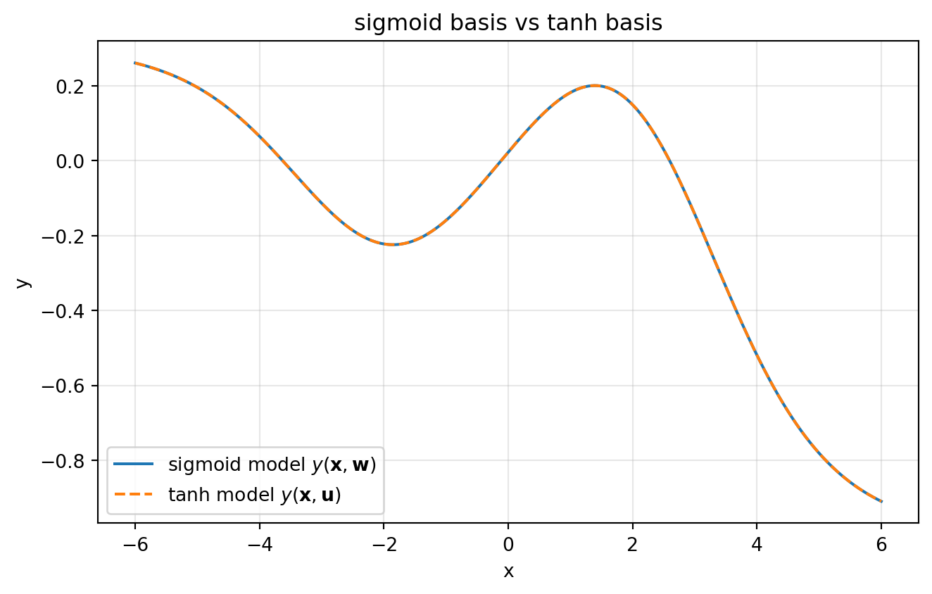

パラメータ変換後の2つのモデルが完全に一致することが確認できた．

Note

数学的には等価であっても，浮動小数点演算では \(\sigma(a) \to 1\)（または \(0\)）と \(\tanh(a) \to \pm 1\) に到達する速さが異なる
\(\tanh\) は引数が \(\sigma\) の半分のスケール（\(a/2\) vs \(a\)）で評価されるため，同じ入力 \(a\) に対して飽和が遅く，勾配情報がより長く保たれる