import torch
import torch.nn as nn
import torch.optim as optim
# --- サンプリング ---
np.random.seed(42)
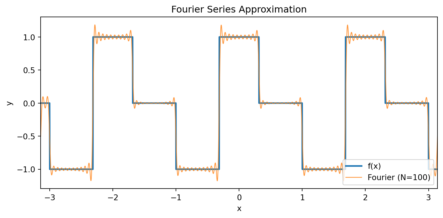
def f_periodic_vec(x):
x = ((x + 1) % 2) - 1
y = np.zeros_like(x)
y[x < -np.pi / 10] = -1
y[(x >= -np.pi / 10) & (x < np.pi / 10)] = 1
y[x >= np.pi / 10] = 0
noise = np.random.normal(0, 0.1, size=x.shape)
return y + noise
K = 5 # フーリエ特徴量の次数
def make_features(x, K=K):
"""sin(kπx), cos(kπx) for k=1..K → 2K次元の特徴量"""
feats = []
for k in range(1, K + 1):
feats.append(np.sin(k * np.pi * x))
feats.append(np.cos(k * np.pi * x))
return np.stack(feats, axis=1)
x_train = np.random.uniform(-np.pi / 2, np.pi / 2, 10000)
y_train = f_periodic_vec(x_train)
X = torch.tensor(make_features(x_train), dtype=torch.float32)
Y = torch.tensor(y_train, dtype=torch.float32).unsqueeze(1)
model = nn.Sequential(
nn.Linear(2 * K, 4 * K),
nn.BatchNorm1d(4 * K),
nn.ReLU(),
nn.Linear(4 * K, K),
nn.BatchNorm1d(K),
nn.ReLU(),
nn.Linear(K, 3),
nn.BatchNorm1d(3),
nn.ReLU(),
nn.Linear(3, 1),
)
for m in model:
if isinstance(m, nn.Linear):
nn.init.kaiming_normal_(m.weight, nonlinearity="relu")
nn.init.zeros_(m.bias)
criterion = nn.MSELoss()
optimizer = optim.AdamW(model.parameters(), lr=3e-3, weight_decay=1e-4)
# --- ミニバッチ学習 + OneCycleLR ---
dataset = torch.utils.data.TensorDataset(X, Y)
loader = torch.utils.data.DataLoader(dataset, batch_size=512, shuffle=True)
n_epochs = 60
scheduler = optim.lr_scheduler.OneCycleLR(
optimizer, max_lr=1e-2, epochs=n_epochs, steps_per_epoch=len(loader)
)
# --- プロット用の準備 ---
xs_plot = np.linspace(-np.pi, np.pi, 500)
fx_plot = np.array([f_periodic(x) for x in xs_plot])
X_plot_tensor = torch.tensor(make_features(xs_plot), dtype=torch.float32)
# --- 学習ループ(各epochのスナップショットを記録) ---
snapshots = {}
all_losses = []
for epoch in range(n_epochs):
model.train()
epoch_loss = 0.0
for xb, yb in loader:
pred = model(xb)
loss = criterion(pred, yb)
optimizer.zero_grad()
loss.backward()
torch.nn.utils.clip_grad_norm_(model.parameters(), 1.0)
optimizer.step()
scheduler.step()
epoch_loss += loss.item() * len(xb)
epoch_loss /= len(dataset)
all_losses.append(epoch_loss)
model.eval()
with torch.no_grad():
snap = model(X_plot_tensor).squeeze().cpu().numpy()
snapshots[epoch] = snap.copy()
if epoch % 10 == 0:
print(f"epoch {epoch:3d} loss={epoch_loss:.6f}")
# --- Plotly (frames + slider) ---
import plotly.graph_objects as go
from plotly.subplots import make_subplots
fig = make_subplots(
rows=1,
cols=2,
subplot_titles=["Training Loss", "NN Approximation"],
horizontal_spacing=0.12,
)
# trace 0: loss曲線
fig.add_trace(
go.Scatter(
x=list(range(n_epochs)),
y=all_losses,
mode="lines",
name="loss",
line=dict(color="#1f77b4"),
),
row=1,
col=1,
)
# trace 1: 現在epochマーカー(赤丸)
fig.add_trace(
go.Scatter(
x=[0],
y=[all_losses[0]],
mode="markers",
name="current epoch",
marker=dict(color="red", size=12),
showlegend=False,
),
row=1,
col=1,
)
# trace 2: f(x)
fig.add_trace(
go.Scatter(
x=xs_plot,
y=fx_plot,
mode="lines",
name="f(x)",
line=dict(color="black", width=2),
),
row=1,
col=2,
)
# trace 3: NN出力(frameで更新)
fig.add_trace(
go.Scatter(
x=xs_plot,
y=snapshots[0],
mode="lines",
name="NN",
line=dict(color="#d62728", width=2),
),
row=1,
col=2,
)
# --- frames ---
frames = []
for ep in range(n_epochs):
frames.append(
go.Frame(
data=[
go.Scatter(x=[ep], y=[all_losses[ep]]),
go.Scatter(x=xs_plot, y=snapshots[ep]),
],
traces=[1, 3],
name=str(ep),
)
)
fig.frames = frames
# --- slider ---
sliders = [
dict(
active=0,
currentvalue=dict(prefix="epoch: "),
pad=dict(t=30),
steps=[
dict(
args=[
[str(ep)],
dict(mode="immediate", frame=dict(duration=0, redraw=True)),
],
method="animate",
label=str(ep),
)
for ep in range(n_epochs)
],
)
]
# --- play / pause ---
updatemenus = [
dict(
type="buttons",
showactive=False,
x=0.0,
y=-0.15,
xanchor="left",
buttons=[
dict(
label="▶",
method="animate",
args=[
None,
dict(frame=dict(duration=100, redraw=True), fromcurrent=True),
],
),
dict(
label="◼",
method="animate",
args=[
[None],
dict(frame=dict(duration=0, redraw=True), mode="immediate"),
],
),
],
)
]
fig.update_xaxes(title_text="epoch", row=1, col=1)
fig.update_yaxes(title_text="MSE loss", type="log", row=1, col=1)
fig.update_xaxes(title_text="x", range=[-np.pi, np.pi], row=1, col=2)
fig.update_yaxes(title_text="y", range=[-1.5, 1.5], row=1, col=2)
fig.update_layout(
height=500,
width=1000,
sliders=sliders,
updatemenus=updatemenus,
margin=dict(t=40, b=80),
)
fig.show()