5  Legends(凡例)

Legendsとは？

Definition 5.1 Legends

• 可視化要素の意味を示すために用いられるコンポーネント
• Labelsと異なり，図の外側にまとめて表示される
• Legends項目を示すマーカーと対応するラベルのセットによって構成される

凡例の位置

凡例の順番

Rules

• Sequential dataについてのLegendsは必ず降順(higest to lowest)にすること
• categorical classについても可視化オブジェクトの目線の順番と整合的な表示順番にすること

categorical classにおける凡例の順番

import yfinance as yf
import matplotlib.pyplot as plt
import pandas as pd

# okabe_ito_colorsの取得
okabe_ito_colors = [
    "#000000", "#E69F00", "#56B4E9", "#009E73",
    "#F0E442", "#0072B2", "#D55E00", "#CC79A7"
]

# 銘柄のシンボル（ティッカー）
symbols = {"Meta": "META", "Alphabet": "GOOGL", "Microsoft": "MSFT", "Apple": "AAPL"}

# 期間設定
start_date = "2020-01-01"
end_date = "2024-01-01"

# --------------------------------------------------------
# Bad plot
# --------------------------------------------------------
# 株価データの取得とプロット
plt.figure(figsize=(12, 8))

# (index, (key, value))形式
for c_index, (name, ticker) in enumerate(symbols.items()):
    data = yf.download(ticker, start=start_date, end=end_date, auto_adjust=True,  progress=False)
    data = data / data.iloc[0] * 100
    plt.plot(data["Close"], label=name, color=okabe_ito_colors[c_index])

# remove box
for spine in plt.gca().spines.values():
    spine.set_visible(False)

plt.title("Stock Prices (2023)")
plt.xlabel("Date")
plt.ylabel("Normalized Close Price (Base=100)")
plt.legend()
plt.grid(axis='y', alpha=0.5)
plt.tight_layout()
plt.show()

# --------------------------------------------------------
# Better plot
# --------------------------------------------------------
# 空のDataFrameを用意
df_all = pd.DataFrame()

for name, ticker in symbols.items():
    # データ取得
    data = yf.download(ticker, start=start_date, end=end_date, auto_adjust=True, progress=False)
    
    # 終値を正規化（初日の価格を100に）
    normalized = data['Close'] / data['Close'].iloc[0] * 100
    
    # 列名に銘柄名を設定してDataFrameに格納
    df_all[name] = normalized

# 最新日のデータ取得（インデックスは日付）
last_day = df_all.index[-1]

# 最新日の値を降順でソート（大きい順）
sorted_columns = df_all.loc[last_day].sort_values(ascending=False).index

# 並び替えた順でプロット
plt.figure(figsize=(12, 8))
for c_index, col in enumerate(sorted_columns):
    plt.plot(df_all.index, df_all[col], label=col, color=okabe_ito_colors[c_index])

# remove box
for spine in plt.gca().spines.values():
    spine.set_visible(False)

plt.title("Normalized Stock Prices(Base=100 at 2020-01)", fontsize=22)
plt.xlabel("Date", fontsize=18)
plt.ylabel("Normalized Close Price", fontsize=18)
plt.xticks(fontsize=14)
plt.yticks(fontsize=16)
plt.legend(fontsize=18, frameon=False)
plt.grid(axis='y', alpha=0.5)
plt.tight_layout()
plt.show()

Bad Example: Legendがunsortedのまま

Better Example: Legendがsortedされている

凡例とシンボル

Rules

• 色だけでなくてシンボルと組み合わせてクラスターの識別力を上げる
• marker colorの区別が難しい場合は，色の順番を工夫すること

import seaborn as sns
from sklearn.datasets import load_iris
import matplotlib.colors as mcolors

# Function to lighten a hex color
def lighten_color(color, amount=0.5):
    c = mcolors.to_rgb(color)
    # linear interpolation towards white
    lightened = [1 - amount * (1 - x) for x in c]
    return lightened

# Load iris dataset
iris = load_iris()
df = pd.DataFrame(iris.data, columns=iris.feature_names)
df['species'] = pd.Categorical.from_codes(iris.target, iris.target_names)

# Okabe-Ito color palette (colorblind-friendly)
okabe_ito = ["#E69F00", "#56B4E9", "#009E73"]

# Set seaborn style
sns.set(style="white")

# Create scatter plot
plt.figure(figsize=(12, 8))
sns.scatterplot(
    data=df,
    x='sepal length (cm)',
    y='sepal width (cm)',
    hue='species',
    style='species',
    palette=okabe_ito,
    s=160,  # marker size
    edgecolor='w',  # white edge to markers
    linewidth=1,
)

# Axis labels
plt.xlabel('sepal length')
plt.ylabel('sepal width')

# Legend style: italic labels
leg = plt.legend()
for text in leg.get_texts():
    text.set_fontstyle('italic')

plt.tight_layout()
plt.show()


# Okabe-Ito color palette (colorblind-friendly)
okabe_ito2 = ["#56B4E9", "#E69F00", "#009E73"]

# Markers for species: circle, square, diamond (angled square)
markers = ['o', 's', 'D']

# Set seaborn style
sns.set(style="whitegrid")

# Create scatter plot
plt.figure(figsize=(12, 8))
# Plot each species separately
for i, species in enumerate(df['species'].cat.categories):
    data = df[df['species'] == species]
    edge_col = okabe_ito2[i]
    face_col = lighten_color(edge_col, amount=0.8)  # lighter fill
    plt.scatter(
        data['sepal length (cm)'],
        data['sepal width (cm)'],
        label=species,
        marker=markers[i],
        s=110,
        edgecolor=edge_col,
        facecolor=(*face_col, 0.5) ,
        linewidth=0.8,
    )

plt.xlabel('sepal length', fontsize=18)
plt.ylabel('sepal width', fontsize=18)
plt.xticks(fontsize=14)
plt.yticks(fontsize=16)

# Legend outside plot on the right
leg = plt.legend(
    fontsize=16, 
    loc='center left',       # legend location relative to bbox_to_anchor
    bbox_to_anchor=(1, 0.5), # x=1 means just outside right edge, y=0.5 is vertical center
    borderaxespad=0.5,
    frameon=False,
    handlelength=3,     # longer marker in legend
    handletextpad=0.05,  # more space between marker and text
    labelspacing=1.2    # more vertical spacing between items
)

# remove box
for spine in plt.gca().spines.values():
    spine.set_visible(False)

plt.tight_layout()
plt.show()

Default Cluter plot

Improved Cluster plot

凡例のタイトル

Rules

• 凡例タイトルは必ずしも必要ではない
• 含める場合には，「凡例」や「キー」といった一般的なタイトルを使うのではなく，ラベル付けされたデータの意味を伝えるタイトルを使うこと

凡例は本当に必要なのか？

Rules

• 凡例がなくて済むなら，凡例は用いないこと
• 明示的な凡例がなくても，各可視化要素が何を意味しているのかが一目でわかるようにする

凡例があると，可視化オブジェクトの読み手は，「１回目線を凡例に向けてから，再びline plotに目線を向けて各線を解釈する」というメンタルワークを結果的に強いられることになります．可視化オブジェクトが凡例なしで済むならば，このような理解の手間を減らすことができます．

この設計の実現手段として「Direct Labeling」があります．

Definition 5.2 Direct Labeling

図の中に適切なテキストラベルや他の視覚的ガイド要素を直接配置する手法

# プロット
plt.figure(figsize=(12, 8))
for c_index, col in enumerate(sorted_columns):
    plt.plot(df_all.index, df_all[col], label=col, color=okabe_ito_colors[c_index])
    
    # direct label を末尾に追加
    y_pos = df_all[col].iloc[-1]
    plt.text(df_all.index[-1], y_pos, f" {col}", color="#1A1A1A",
             va='center', fontsize=20)

# remove box
for spine in plt.gca().spines.values():
    spine.set_visible(False)

plt.title("Normalized Stock Prices (Base=100 at 2020-01)", fontsize=22)
plt.xlabel("Date", fontsize=18)
plt.ylabel("Normalized Close Price", fontsize=18)
plt.xticks(fontsize=14)
plt.yticks(fontsize=16) 
plt.grid(axis='y', alpha=0.5)
plt.tight_layout()
plt.show()

Density Plot without Legends

• text label colorが明るすぎると，ラベルの読みづらくなるので，色の対応をキープする範囲内で暗い色にする

from cmap import Colormap
import numpy as np

def darken_color(rgb, amount=0.7):
    # rgb is tuple (r, g, b, a), scale RGB channels by amount (0 < amount < 1)
    r, g, b, a = rgb
    r, g, b = np.array([r, g, b]) * amount
    return (r, g, b, a)


# Iris データセットをロード
iris = load_iris()
df = pd.DataFrame(data=iris.data, columns=iris.feature_names)
df['species'] = pd.Categorical.from_codes(iris.target, iris.target_names)

# カラーマップ（手動でセット）
cm = Colormap('okabeito:okabeito')  # case insensitive
mpl_cmap = cm.to_mpl()
colors = [mpl_cmap(i) for i in np.linspace(0, 1, 5)][1:]
darker_colors = [darken_color(c, amount=0.5) for c in colors]

palette = dict(zip(df['species'].cat.categories, colors))

# Set Seaborn style
sns.set(style="white")

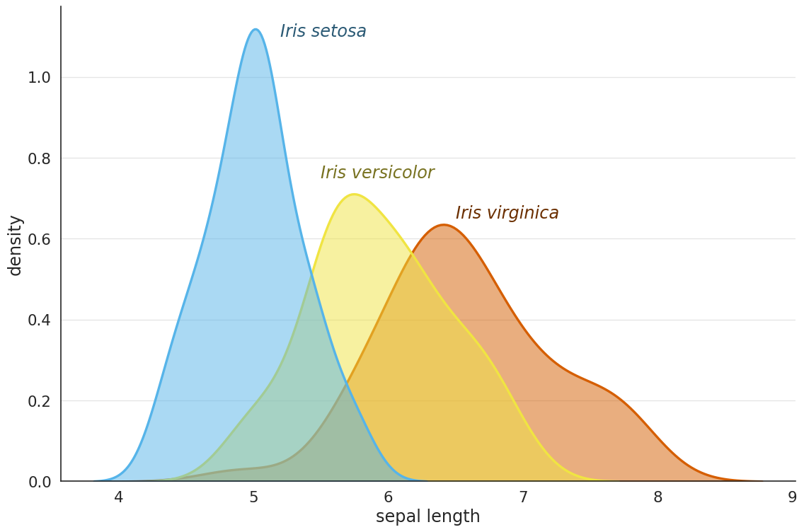
# カーネル密度推定プロット
plt.figure(figsize=(12, 8))
sns.kdeplot(
    data=df,
    x="sepal length (cm)",
    hue="species",
    fill=True,
    common_norm=False,
    palette=palette,
    alpha=0.5,
    linewidth=2.5
)

# ラベルのスタイル
plt.text(5.2, 1.1, "Iris setosa", color=darker_colors[0], fontsize=18, style='italic')
plt.text(5.5, 0.75, "Iris versicolor", color=darker_colors[1], fontsize=18, style='italic')
plt.text(6.5, 0.65, "Iris virginica", color=darker_colors[2], fontsize=18, style='italic')

# 軸ラベルと体裁
plt.xlabel("sepal length", fontsize=18)
plt.ylabel("density", fontsize=18)
plt.xticks(fontsize=16)
plt.yticks(fontsize=16)
plt.legend([],[], frameon=False)  # 凡例を削除
sns.despine()  # 枠線を削除
plt.tight_layout()
plt.grid(axis='y', alpha=0.5)
plt.show()